The Workspace is the main RiverWare window and the main interface used to view, run, and investigate the model.

The workspace features a main menu bar in which the various functions of RiverWare are organized into menus. The workspace also contains a dockable toolbar featuring shortcut buttons to some key RiverWare operations and utilities. There is also a dockable object listview window of all the objects on the workspace. A screenshot of the workspace is shown in Figure 1.1.

 

The workspace supports two modes

Typically, Full mode is used when building a model or investigating objects on the workspace. Compact mode is used when you don’t need to see the canvas views and you want to use the toolbar buttons and menus to run a script, execute a run or look at outputs. In this approach, some users will open RiverWare, detach the Object List and then switch to Compact mode to provide a more efficient use of screen space.

To switch between the two modes:

The following sections describe each mode.

When the canvas is shown if Full mode, the canvas views are shown along with the menus, toolbar, dockable windows, and status bar. This is the default and primary view of the simulation space where models are built and modified. In the workspace, a model is graphically represented as a network of objects with links connecting the objects. The workspace allows for exploration of the model through the following viewing options:

Figure 1.3 shows a view of the workspace in Full mode.

“Compact” display mode shows only the title bar, menus, toolbar (if enabled), and status bar. In other words, the Compact display mode hides the canvas/views, Simulation Object List (if shown and docked within the workspace), and Animation controls (if shown and docked within the workspace). Figure 1.4 shows a view of the workspace in Compact mode.

You can select the icon that is shown at the left of the title bar on all windows associated with the RiverWare session. The ability to control the color of the RiverWare icon is particularly useful when you are comparing two models in two separate sessions of RiverWare. There are two ways to change the icon:

Then all windows and the task bar will use the selected icon. The selected icon color is saved in the model file.

Figure 1.5, Figure 1.6 and Figure 1.7 show the available icons.

Sometimes the workspace can obscure other dialogs that you may wish to see. When this happens, you can use the Send Workspace to Back operation to force the Workspace window to be displayed behind any other overlapping window. The action is available in the following ways:

The font, size and style used for menus, lists and other text can be changed from the Utilities, then Windows, then Set Font menu. Following are limitations with this feature:

The toolbar in RiverWare is dockable, meaning it can be moved from one side of the workspace to the other or exist as an independent dialog. Table 1.1 summarizes the Workspace buttons.

The Object Viewer button allows for quick access to the Object Viewer with previously opened objects. It is disabled if there are no objects shown in the viewer. See “Object Viewer and Open Object Dialogs” for details.

Also shown are color-coded icons for the following:

Hover over any icon for a tooltip indicating the location or click to open that set. Also, the sets are still available through the Policy menu. See “Types of RPL Sets” in RiverWare Policy Language (RPL) for the color code for sets.

The Simulation Workspace right-click context menu (when not selecting a simulation object icon) has the following options.

The moving of Simulation Object icons on the Workspace can be disabled by locking icon positions as follows:

RiverWare provides the option to show commas as a thousands separator in slot values (slot dialogs, SCT, accounts, and exchanges) and numeric values entered into a RPL expressions. Commas are shown by default but can be turned off by selecting the Workspace, then Show Commas in Numbers option. When the option is selected, all values will update automatically.

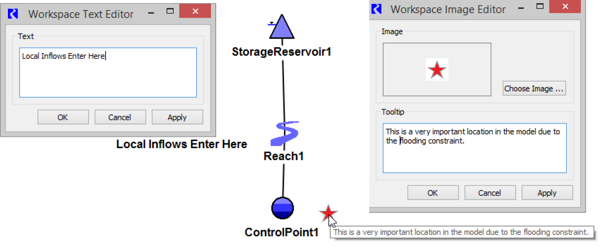
Often users find that they may wish to annotate their workspace with text or image files. To do so, use the right-click context menu and select Add Text or Add Image. This opens a dialog where you can specify the text or an image, respectively. The image on the left shows the text editor and the resulting text below it. Figure 1.9 shows the image editor with a small image shown. Also shown is the tooltip for the specified text. This is the text you see when you hover over the image.

These are supported separately on the Simulation and Accounting views, but not the Geospatial view.

Images are saved in the model file and will increase the model file size. GIF, PNG, or JPG images are supported.

The Output Canvas allows you to create spatially distributed output visualization diagrams. You can show the following items from an Output Canvas directly on the Simulation and/or Geospatial Views. See “Showing Canvas Items on the Workspace” in Output Utilities and Data Visualization for details.

When items are shown on workspace views, an additional panel of Animation Controls is shown below the Simulation Object List, as shown in Figure 1.10. See “Animation” in Output Utilities and Data Visualization for details on the controls.

Like other dockable windows, this panel can be pulled off the workspace to its own dialog, docked on the left side of the workspace or closed. To redisplay the panel, use the Utilities, then Windows, then Show Animation Controls menu.

The Slot Cache provides a temporary copy of series slot values. The cache is created from the Workspace, then Create Slot Cache menu. Within the run range, all visible series slots (except those on Data Objects that are not optimization variables, exchanges, supplies, and those slots with different step size than the run) are copied to the cache when this menu is operated. These values can be accessed using RPL predefined functions SlotCacheValue and SlotCacheValueByCol. They are typically used during an optimization run for certain Seed Method parameters. The cache values are not saved in the model file.

Manually clear the Slot Cache using the Workspace, then Clear Slot Cache option.

All objects can be cleared from the workspace by selecting Workspace, then Clear Workspace. A confirmation dialog appears warning that all objects on workspace will be removed. All rulesets will also be cleared and any unsaved changes will be lost.

Large models can rarely be viewed in their entirety on the workspace, making it difficult to locate objects. There are, however, multiple ways of navigating through a model on the workspace or locating particular objects within a model. These methods are described in greater detail below.

At 100% zoom level, object icons are shown in their natural size of 40x40 pixels. When zooming out, e.g. to 50%, to expose a broader area of the workspace, the object icons and labels are also zoomed out and their size is reduced. When zooming in beyond the 100%, icons, labels and links remain their natural size (100%) instead of becoming larger (or thicker links). This allows you to expose more detail of background images around closely clustered objects without showing large icons. This implementation of smart zooming affects only the Simulation and Geospatial views.

An overview of a model can be accessed with the locator view. The locator view displays the entire workspace on a miniature scale. The locator view is accessed as follows:

The rectangle represents the current displayed portion of the workspace. Dragging the rectangle to different regions of the model in the locator view will cause that region to be displayed on the workspace.

A status bar shows the name of the Simulation Object near the cursor. This functions even while dragging the inscribed rectangle.

The Locator View implements a Context Menu (right-click) with the following options:

In-view Locator Mode is an alternative to the separate Locator View.

Selecting this mode causes the workspace to temporarily rescale to show the scope of all of the simulation objects on the workspace. The rectangular region of the normally visible area (at the currently set zoom level) is shown as a shaded rectangle. Drag the shaded rectangle to a new area and upon releasing the button, the workspace is positioned at the new area at the previous zoom level. This allows you to quickly snap to a different area in your model.

If a model is not particularly large or is familiar, it is possible to move to the desired region of the model using the scroll bars. By default, the scroll bars are located in the lower corners of the workspace. Adjusting the scroll bars will pan the model to the desired location. Also, you can use the middle button to temporarily enter Pan Mode to pan through the workspace.

The dockable object list window provides the most comprehensive means of locating a specific object within a model. The object list window can be detached from the workspace and be positioned at a desired location. If you undock and/or close the object list, you can show it using the Utilities, then Windows, then Show Simulation Object List menu. Selecting the desired object in the listview window automatically selects the object on the workspace. Right-clicking an object allows you to open the object without scrolling the workspace.

Objects in the list window can be organized by Name, Type, Position or a Custom Order. Objects are further organized in ascending or descending order by selecting the column label.

The Custom Order is defined using the Edit Custom Order menu. The Edit Custom Object Order dialog is shown:

Set an initial order using the Name, Type, or Position buttons. Then select one or more objects by selecting an object and then using Shift or Ctrl key and selecting another object. Drag and drop or use the up and down arrow buttons to rearrange. When you click OK, this order is preserved as the custom order and is shown on the Object List.

You can configure the workspace appearance when the model is first opened in terms of the view, zoom, and scroll location. On the workspace, use the Workspace, then Initial Appearance menu. The Initial Workspace Appearance dialog opens.

First, choose one of the following:

Then, for each of the three workspace views, Simulation, Accounting (when enabled), and Geospatial, specify the zoom level and scroll location to use. Each view maintains these setting separately. For the location, select between one of the following methods to specify where to scroll:

The DateTime can be specified explicitly or symbolically as RPL DATETIMES; see “DATETIME” in RiverWare Policy Language (RPL) for details. Text below the editor field indicates the actual DateTime of the entered symbolic time text (if it is valid), or the status if it is not valid. You can also use the menu to specify one of the common DateTimes. Some of these are expressions which must be edited to become valid, e.g. by replacing “N” with a nonnegative integer and the HH:00 MMM DD, YYYY formula, where you substitute the hour, month, day and year.

The Datetime Editor option opens a separate dialog to specify the DateTime using a selector configured for the model's timestep size.

The Global RPL Function option opens a Function Selector to select a RPL function in the Expression Slot or Global Function Set.

Select Help (question mark icon button) on the right side of the symbolic DateTime editor to show a description of symbolic DateTime representations.

The Workspace has two cursor selection modes. These define the effect of clicking and dragging on the workspace.

Selection Mode is used for selecting and repositioning Simulation Object icons on the workspace.

Multiple icons can be selected by dragging a rectangle over the icons (with the drag operation started off any icon). Selecting an icon while holding down the Control key toggles the icon in or out of the selected set.

A set of selected icons can be moved together by starting the icon drag on one of the selected icons. An icon move operation can be aborted by hitting the Esc (escape) key before releasing the button.

Pan Mode allows the user to move or pan the workspace canvas within the visible workspace area.

Use the middle mouse button to temporary enter Pan Mode from Selection Mode.

Then the Close Dialogs button closes the selected types. This utility never closes the Workspace. In addition, the following types of dialogs are just minimized instead of being closed:

The canvas is the region within the workspace in which models are built and displayed. These canvas is shown when in Full mode, but not shown in Compact mode, as described in “Workspace Display Mode”.

There are three versions of the canvas which display different Views of the objects and connection. The Simulation View displays a schematic of the basin; objects are linked together to form a network. The Accounting View (when accounting is enabled) shows a similar schematic, but each object is displayed as a rectangle which contains all the accounts on that object. The third view, the Geospatial View, displays objects at their actual locations on a georeferenced background map. Because of the differences in how the network is displayed in each view, there are different configuration options for each canvas. The following sections describe each canvas and the configuration options.

The Simulation View displays a schematic of the basin; objects are represented by icons and are linked together to form a network.

The canvas properties dialog is accessed as follows:

This dialog allows you to change the following attributes of the canvas:

The Simulation Workspace supports the ability to show an image loaded from an image file (JPEG or PNG) as the background. The utility is accessed by right-selecting the workspace and choosing Background Image.

The path of the selected image is preserved in the model file (if the model file is saved after configuring the background image). When loading a model with a configured background image file, if the background image file does not actually exist at the recorded path, the model loads without a problem, and the currently-invalid image file path is retained.

If the selected image file does not represent a valid, supported image file format, the thumbnail (small image preview) will be blank, and the Tooltip on the thumbnail will indicate an error. Figure 1.15 illustrates.

Configurable background image properties include the following:

A typical use of a background image is a map. This works well if you can reasonably position the icons at approximate positions and/or you do not have or wish to use geospatial coordinate data. But, georeferencing is available on the Geospatial View; see “Geospatial View” for details.

If Accounting is enabled, the accounting network is displayed in the Accounting View, and can be selected by the option menu on the toolbar. The accounting view provides a representation of the physical objects, as well as the accounts on those objects where the network can be displayed without occluding or modifying the original physical network.

General configuration of the accounting view is identical to the Simulation View. See “Canvas Properties” for details.

See “Accounting Network” in Accounting for details on the Workspace Accounting View.

The Geospatial View of the workspace provides a spatially coherent display of the modeled basin by associating a map projection and its Cartesian coordinate system with the view. Users locate objects and a background map image in this coordinate system, allowing RiverWare to display a schematic view of the modeled basin overlaid in registry with the map. That is, RiverWare objects are displayed at their location on the map. By providing an intuitive and information-rich view of a basin, the Geospatial view complements the Simulation and Accounting views of the workspace.

Following are key features of the Geospatial View.

Graphical information systems (GISs) support storage, analysis, and display of spatial data. This section introduces some basic GIS terminology and concepts which are relevant to the Geospatial View.

Locations on the spherical earth are most often represented as a pair of coordinates representing latitude and longitude. For some applications, a third coordinate representing an elevation relative to mean sea level is also used. To display a part of the curved surface of the earth on a flat surface necessarily requires a projection, and GIS systems typically represent flat display locations as Cartesian coordinates in a plane onto which the surface of the globe has been projected.

Several standards have been developed to provide agreed-upon coordinate systems for a given area. These standard coordinate systems define a set of map projections which together cover the target area. One common coordinate system which covers the globe is the Universal Transverse Mercator (UTM) coordinate system. This system defines a projection for the northern and southern areas of each of 60 longitudinal zones spanning the globe. For example, in the projection UTM Zone 11 North, the coordinates eastings = 397,800 m, northings = 4,922,900 m, corresponds to a location in central Oregon, USA.

Another standard coordinate system is the State Plane coordinate system which defines a set of projections for the United States. In this system, each state is divided into one or more zones, so a location is specified by a state, zone designation, and x, y coordinates.

Coordinates, whether they be geographic (latitude and longitude) or correspond to a map projection, are specific to a datum. A datum is a reference surface and surveyed coordinates for a set of actual points and lines. Examples of common datums include the North American Datum of 1983 (NAD83) and the World Geodetic System of 1984 (WGS84).

The Geospatial View has a map projection associated with it, and everything displayed in that view (e.g., object icons, background image) needs to be displayed in that projection. Because RiverWare assumes that a single projection is shared between the Geospatial View, the object coordinates, and the map, RiverWare does not need to know the mathematical details of that projection. However, if these details are provided to RiverWare (typically by providing a background image which contains metadata describing the image’s projection), then RiverWare can translate projected coordinates to geographic coordinates, and display these coordinates where appropriate.

To support the Geospatial View of the workspace, RiverWare associates coordinates in the view’s projected coordinates system with each object on the workspace. To provide more flexibility for the user, RiverWare supports both Actual and Display spatial coordinates. Actual coordinates are the static coordinates of the object which may come from other sources. The display coordinates are the location where the object is shown on the geospatial view. Often the display coordinates differ from the actual coordinates because the object was moved slightly for less icon clustering or better display.

When an object is created, it is placed at the point of creation in the current view and given locations in the other two views based on its location in the current view. Objects can be moved in any view, and in the Geospatial View this will change the display spatial coordinates. This view also provides the following additional mechanisms to edit or specify spatial coordinates:

Following is a description of the Object Coordinate Manager Dialog which is used to edit/view object coordinates. The Object Coordinate Manager is non-modal and accessed by right-selecting the main workspace (in the Geospatial View) and then selecting Object Coordinates.

The Object Coordinate Manager dialog displays both the display and actual spatial coordinates for all workspace objects. This dialog supports editing of individual fields as well as cut/paste/copy. For each object, both the display and actual spatial coordinates are displayed.

Following are operations that you can perform through the dialog.

Figure 1.17 illustrates the possible movement of coordinate data within RiverWare.

This section describes how you might begin to use the Geospatial View with an existing model which to this point has made use of only the Simulation and/or Accounting Views. Figure 1.18 shows the workspace Simulation View for the model we will be using to illustrate this process.

The Geospatial View is most useful when a basin map exists which can be located (georeferenced) in a known projection system. If this information is not available, consider using the Simulation View with a background image.

The Geospatial Canvas Configuration Dialog allows you to specify information about your georeferenced image and how it relates to the RiverWare workspace. It is accessed as follows:

We will discuss each of the Geospatial Canvas Configuration Dialog tabs in turn.

This portion of the dialog describes the background image and the projected and geographic coordinate systems associated with that image (and the Geospatial View in general).

Image files are specified by full path names with environment variable expansion. Environment variables are specified using the $PATH syntax. If the image changes outside of RiverWare you may need to reload it using the Reload button.

Of the many image formats supported by RiverWare¹, the most common are JPEG, PNG, JPEG 2000, GeoTIFF, and MrSID.When an image is loaded, RiverWare checks for the presence of two type of useful metadata:

If present, these data are used to set appropriate aspects of the configuration. Some image formats support the embedding of these metadata in the image file itself (e.g., GeoTIFF, JPEG 2000, and MrSID), but RiverWare also checks for a co-located file with a suffix indicating that it contains image metadata. For example, RiverWare will look for an associated file in the world file format, a plain text file format developed by ESRI for georeferencing raster map images.

A valid world file contains six lines, each containing a floating point value, denoted here by the letters A to F. These values define an affine transformation from pixel coordinates to projection coordinates in the form:

For many GIS applications, creating an image with a world file is relatively straightforward. For example, to do this in ArcMap 10.0, select File, then Export Map, then select the Write World File checkbox in the dialog. On the other hand, when this is not possible, the world file format is simple enough that it can be created by hand with a text editor.

The Geospatial View currently supports only images with unrotated, square pixels, thus not all map images can be displayed as background images. If metadata indicate that these assumptions are violated, RiverWare will notify the user at image load time.

Following are additional controls and information contained in this section of the dialog:

This panel displays information about the projected and geographic coordinate systems associated with the Geospatial View.

You can either set these fields interactively or, if the appropriate image projection metadata is present, RiverWare will set them automatically.

The geographic coordinate system portion of this panel is only relevant when full projection information is present, typically part of the projection metadata. When this information is not present, this portion of the panel is disabled.

This panels displays information about the locations of the background image and canvas in the projected coordinate system.

To display the background image at the proper location on the canvas, RiverWare needs to know its location in the projected coordinate system (i.e., the image must be georeferenced). There are two alternatives for providing this information if RiverWare did find it when the image was loaded. One is to select the Set from: World File button. RiverWare will then present a file chooser dialog for specifying the world file containing the image’s georeferencing information. This option is appropriate when an appropriate world file exists, but it is either not co-located with the image or has an unusual name that prevents RiverWare from discovering it.

If no metadata is available, then another option is to provide coordinates for two specific locations in the map, in which case RiverWare will use these reference point coordinates to compute projection coordinates for the full image. To provide this information to RiverWare, select the Set from: Reference Points button. This opens the Image Location Dialog which displays a view of your image. For this utility, a reference point is a location for which you know the coordinates and you can locate in the image. Only 2 reference points are needed to locate the image in the projection coordinate system.

As shown in Figure 1.24, you perform the following steps.

If you have set the background image rectangle location interactively, you can export the corresponding georeferencing information by selecting the Export World File button. RiverWare will allow you to select a file name and write the background image’s georeferencing information to that file in the world file format. This file can then be used to automatically register the image within other RiverWare models or with any application that can supports the world file format.

In the Canvas Rectangle Location area, you specify where the canvas rectangle lies in the projection’s coordinate system, by giving the coordinates of the lower left and upper right corners of that rectangle. Checking the Set from Background Image withe Margin checkbox will cause RiverWare to automatically compute the canvas location to be that of the Background Image with an optional margin added to each side. Clearing this box allows you to interactively enter three coordinates of the canvas location (the remaining coordinate will be computed by RiverWare based on the other three). Care should be taken here to enter a canvas location that includes that of the image.

This panel provides a high-level view of the canvas and image rectangles, drawn as rectangles whose size and relationship to each other matches that defined in the Background Image Rectangle Location and Canvas Rectangle Location panels. The locations of each coordinate (A, B, C, and D) are shown in the thumbnail.

In this tab, you can specify additional display settings for the geospatial workspace, as follows:

All selections in this frame are applied to the sample reservoir icon immediately, but are applied to your workspace when the OK or Apply button is selected.

When you are satisfied with the configuration and would like to apply it to the Geospatial View, select OK or Apply at the bottom of the dialog. This will apply changes from all tabs of the dialog (OK will also close the dialog). If the current spatial coordinates of one or more object do not fall within the configured canvas boundaries, you will be prompted with the warning dialog shown. A detailed explanation can be shown, basically explaining that RiverWare expects all objects to be displayed on the canvas, and that continuing the apply operation will cause RiverWare to automatically reposition those objects so that they are on the canvas. This is a reasonable thing to do if this is the first time an image and coordinate system information has been configured for this view. Once the new configuration has been applied the Geospatial View, you can then refine the positions of the object (by direct manipulation with the workspace or using the Object Coordinate Manager, described below). On the other hand, the objects could have correct coordinates for the coordinates system but are off of the canvas due to unintended changes to the canvas location, in which case you should cancel the apply operation and correct any problems.

Following are some strategies for dealing with overlapping icons which is sometimes called icon clustering.

The workspace displays the objects representing features in the basin. The object icons are a convenient way to visualize the physical layout of a modeled system. These objects also contain the data and the physical process algorithms that drive the simulation. This section describes how to manage objects on the workspace.

Objects are added to the workspace using the object palette. The Palette contains all of the available object types used to represent features of a river basin. It is the source from which objects are instantiated on the workspace. To place objects on the workspace, drag them off the object palette and place them in the desired location on the workspace. You can access the Object Palette as follows:

An object is created by selecting its icon and dragging it off the Palette onto the workspace. At the time an object is created, the first timestep and timestep size in Series Slots are matched to the Run Control run time settings. The slots show display attributes (Units, Scale, Precision, and Format); see “Unit Schemes” for details. Default user methods are also selected for new objects. Slots associated with the selected controller and Methods are allocated in memory. See “Object Types” in Objects and Methods for details on each type of object.

To open an object to see its slots, method selections, accounts, and description:

This displays the Object Viewer. See “Object Viewer and Open Object Dialogs” for details.

Objects can be selected for various reasons such as moving them, deleting them, or adding them to a subbasin. Once an object or group of objects has been selected, it will be highlighted both on the workspace and in the dockable list window.

The following are ways to select an object on the workspace:

Deleting objects from the workspace by selecting one or more objects, then right-clicking one of them. Select Delete Object from the menu. A confirmation dialog appears to inform that the selected objects will be removed from workspace.

This deletion can also be accomplished by selecting one or more objects and pushing the Delete key or by selecting the objects and then from the main menu select Workspace, then Objects, then Delete Selected Object(s). In both cases, confirmation is still required.

An object can be moved by selecting it and holding down the button while dragging the object to the desired location. This will readjust the links to the object as well. A set of selected objects can be moved while maintaining their relative positions. The selected objects remain visible on the workspace during the move. Moving objects will change the Display Coordinates on the Geospatial view but will not change the Actual Coordinates; see “Object Coordinates” for details.

Objects on the workspace are shown grey when dispatching is disabled. Tooltips indicate the state as well. A sample is shown in Figure 1.25. In this state, the objects will not dispatch, but they will still execute beginning of run checks. Enable or disable dispatching by right-clicking the selected objects and selecting Enable/Disable Dispatching. See “Disabling Dispatching” in Debugging and Analysis for details.

Object Clusters allow you to group together simulation objects on the workspace and show only a single icon.

Clusters have the following properties:

Following is more information on how to create and use Clusters.

To create a new cluster, select one or more simulation object icons on the Simulation or Geospatial workspace and do one of the following:

If any of the selected simulation objects are already in a cluster, the Add to Object Cluster context operation is instead presented as Move to Object Cluster. This operation is used to move objects from one cluster to another.

In general, to modify a cluster you can either right-click the cluster on the workspace, right-click the cluster in the Object List, or select the cluster and use the Workspace, then Object Cluster menu.

Following explains the various options, depending on the selection and the menu chosen, as follows:

To see a list of the objects in a cluster, use one of the following methods to open the cluster.

The Open Cluster Dialog shows the member objects in a list. Sort by object type or object name by selecting the column header. From this dialog, you can do the following:

Most of these operations are also available by right-clicking an object/cluster in the Simulation Object List.

Objects can be exported to a file and then imported into the same or another model. Exporting one or more objects includes exporting slot data, method selections and optionally links, accounts and supplies. Objects can be imported and exported to and from the workspace as follows.

To export, first select, one or more objects. Then select Workspace, then Objects, then Export Object from the main workspace. The user is then presented with the Export RiverWare Simulation Object File dialog, which is used to specify how the objects should be exported and to which file the objects should be written. Figure 1.29 illustrates.

The following options are available for exporting depending on the model and possibly the selected objects’ components.

When exporting objects and links, only those links between exported objects will be written. Similarly, only those supplies between exported accounts will be written. In addition, the following are not exported:

To import, use the Workspace, then Objects, then Import Object menu from the RiverWare workspace. On import, the objects will have the same name as the original object unless an object by the same name already exists in the model. In this case, an integer is added to the object’s name. The following options are available on import.

Imported objects are automatically selected (highlighted). Typically the user will then move all of the imported objects immediately to the desired location by dragging them on the workspace. This is especially true if they are on top of other objects. While the objects are still selected, it may be useful to create a subbasin of these objects so they may be easily selected later. See “Creating New Subbasins” for instructions on creating a subbasin from the selected objects.

Following are the limitations when importing objects. Objects are similar to model files, they can only be imported in models that have the same or higher version number, e.g. an object exported from a RiverWare 5.0 model can only be imported into RiverWare 5.0, 5.1, etc.

On import, the objects will be placed at the same coordinates as the objects in the model from which they were exported in both the simulation and accounting views. If the workspace is too small to accommodate these new objects, the workspace will grow to exactly fit the imported objects (including a small border).

When an object or supply is imported and the name already exists in the model, the newly imported objects will be renamed by adding a number to the end of the name. The supplies will then be renamed using the default supply naming convention, “Object# Account to Object# Account”. A warning message is posted. If this new name is not available, because of multiple supplies between the same two accounts, the word “DUPL” is added to the end of the supply name to make it unique. These supply names can be changed from the account configuration. Accounts should not need to be renamed as account names are not unique only the object names are.

There are a number of scenarios in which import/export of objects could be useful. One such example is when a team of modelers wish to break up a model and have various people work on different components. Following are some tips for this process.

Each team member would take the full model and then pare it down to the desired objects, do the modeling work and then recombine the pieces into one model. To pare down a model, it is typically better to delete unused objects than to export and import the desired objects into another model. By deleting objects, the Run Control parameters--run range, timestep length, controller, settings--are preserved. Also, the output devices, DMIs, object level accounting methods are then available in the pared down model.

To then recombine the model with the original, it is best to delete the objects from the original model and then import the new objects from the pared down version(s). This prevents naming conflicts and having to rename newly imported objects.

Links are the connections between slots on objects which pass information during a simulation run. They propagate a value from a slot on one object to a slot on a different object. Several links may exist between different slots on two objects, but only one line is represented on the workspace. By hovering over the link, all the linked slots are displayed in a tooltip.

There are three utilities for viewing, creating and deleting links: Context Menus, Smart Linker, and Edit Links dialog. See “Editing Links” in Model Building Quick Start for details.

The appearance of links, objects, accounts, and supplies on the workspace can be manipulated using the Display Group Editor. The dialog is accessed as follows:

This brings up a window with the option to select Display Group Properties.The Display Group Editor provides the ability to create groups of links, groups of objects, and if accounting is enabled, groups of supplies and groups of accounts. The display properties and the membership of a group can be changed by double-clicking that group. The membership of the groups need not be mutually exclusive. The groups are prioritized. For example, if two link groups contain the same link, the group highest in the list (lowest priority number) will be used to set the display properties of that link. Display groups can be enabled and disabled by selecting the checkmark in the Enabled column.

The Count column provides information on the number of items in the group of the form XX of YY, where YY is the number of items in the group's set selection, and XX is the number of those items which are governed by that group (i.e. not currently governed by an enabled, superior group).

A link group can be created by selecting Group, then Add Link Group in the Display Group Editor. Double-clicking the new link group entry will bring up the Link Display Group Configuration dialog. Provide a name that will be shown in the Link Group Editor.

In the top part of the dialog, you specify the slots on either end of the links. Select Select Slot(s) in the Slot 1 area to specify the first set of slots. You can use filters and other selection mechanisms to quickly choose a large number of slots. Either leave the Slot 2 as Any Slot or specify slots using the selector. Example 1.1 provides an example. See “Selector Features” for details.

You can then choose to show arrow heads on either end of the links using the Show Arrows option.

In the bottom portion of the dialog, you can control the Line Style, Line Width, and Line Color of the links.

From the Workspace, a link can be added to link group by right-clicking the link(s) between two objects, hovering over the Add to Link Group option, hovering over the desired link (there can be multiple links on the same line between two objects), and selecting the desired Add to: <link group>.

Equivalently, links can be added to a link group within the Display Group Editor. This approach allows multiple links to be added to a link group at once. By double-clicking the desired link group, the Link Display Group Configuration window is opened. The slot on one end of the link is selected by selecting Select Slot(s) in the Slot 1 field. If the Any Slot toggle is selected in the Slot 2 field then all links to any of the slots listed in the Slot 1 field will be associated with the display group. While the Link Display Group Configuration dialog does not display the links associated with a particular group, the slot selector dialog remembers the selected links. Therefore, the user can view the links associated with a group by selecting the Select Slots(s) button. To make a more specific selection of links, slots can be selected in the Slot 2 field if the Selection toggle is enabled. Only those links that are connected to a slot in the Slot 1 field and the Slot 2 field will be associated with the display group.

Two predefined link groups are provided for all models: Main Channel Links, and Default. The Main Channel Links group contains all links between main channel upstream slots and main channel downstream slots. The Default link group contains all links on the workspace.

Supply groups are active only if accounting is enabled. A supply group can be created by selecting Group, then Add Supply Group in the Display Group Editor. Double-clicking the new supply group entry will bring up the Supply Display Group Configuration dialog. The membership of the group and the line style, color, and width of the group members can be set with this dialog. The membership of the group is controlled by selecting the Select Supply(s) button. See “Supply Groups” in Accounting for details on Supply Groups.

Account groups are active only if accounting is enabled. An account group can be created by selecting Group, then Add Account Group in the Display Group Editor. Double-clicking the new account group entry will bring up the Account Display Group Configuration dialog. The membership of the group and the fill style, fill color, account width, account aggregation, and border color of the group members can be set with this dialog. The membership of the group is controlled by selecting the Select Account(s) button. If account aggregation is selected, the selected accounts, on a particular simulation object, will be collapsed into one icon. The icon will appear as a stacked group of accounts to indicate the presence of more than one account. An account can also be added to an Account Display Group by right-clicking the account on the workspace, hovering over Add to Account Group, and selecting the desired Account Display Group. If the account is already a member of an Account Display Group, this option will be replaced with Account Group Membership. Hovering over this option will show the display group to which the account belongs. See “Account Groups” in Accounting for details on Account Groups.

The display options associated with object groups apply to both the Simulation View and the Accounting View of the RiverWare workspace (some options apply only to accounting). An object group can be created by selecting Group, then Add Object Group in the Display Group Editor. Double-clicking the new object group entry will bring up the Object Display Group Configuration dialog. The membership of the group and the fill style, fill color, visibility, drawing layer, and border color of the group members can be set with this dialog. The membership of the group is controlled by selecting the Select Objects(s) button.

An object can also be added to an Object Display Group by right-clicking the object on the workspace, hovering over Add to Object Group, and selecting the desired Object Display Group. If the object is already a member of an Object Display Group, this option will be replaced with Object Group Membership. Hovering over this option will show the display group to which the object belongs. The fill style, fill color, and border color apply only to objects in the Accounting View as indicated in the Object Display Group Configuration dialog. The Drawing Layer option is useful when simulation objects are stacked on top of each other on the workspace. The user can control the order of the layering or stacking by specifying the Drawing Layer. Objects with a higher priority Drawing Layer (lower numerical value) will be displayed on top of objects with a lower priority Drawing Layer.

It is possible to export or print an image of the workspace for use in presentations or other graphic applications.

Selecting File, then Export Workspace Image brings up the options to export the entire workspace image or only the visible portion of the workspace. The image can be saved in the following formats: PNG, BMP, JPG, PMB, PGM, PPM, XMP, or XMB. It is also possible to specify image resolution, width, and height in the export dialog.

In general, users will get the best results if they use PNG instead of JPG. PNG is very much like GIF, but has an open specification. (GIF is proprietary). JPG is lossy, but best for images with a lot of continuous variation. GIF and PNG are non-lossy for images with a limited number of colors (no more than 256 colors, which is the case with RiverWare workspace images, for the most part), and they compress really well for images with large blocks of solid color (also an attribute of the workspace). Also, GIF and PNG are much cleaner for the purpose of workspace and plot images. With JPEG, the user may see jagged edges.

The print option prints the entire workspace image. To print the workspace, select File, then Print, which brings up the Setup Printer dialog. In this dialog, various printing options can be selected.