
Setting Up a Multiple Run Configuration
This section provides the steps to setting up a multiple run configuration. Setting up a multiple run configuration requires specifying several parameters in the MRM Configuration. The parameters and brief descriptions are provided below.
• Open the Multiple Run Control dialog by selecting Control, then MRM Control Panel from the main RiverWare menu bar or select the MRM button on the toolbar.
• Create a new configuration and edit an existing configuration, as appropriate. See Creating a New Configuration and Editing an Existing Configuration for details.
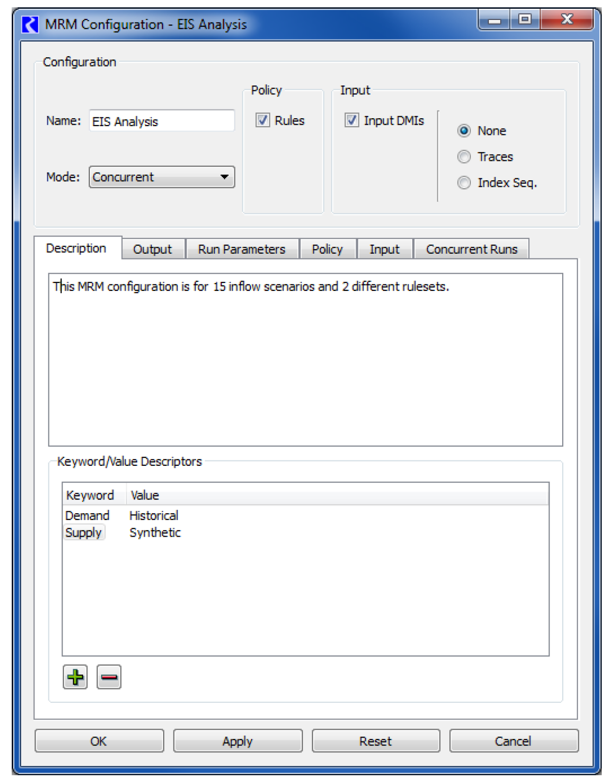
Name
Provide a unique name for the configuration in the Name field.
Description
The configuration description in the upper panel may be multiple lines of text. This first non-blank line of the description appears in an MRM output RDF file. This text is optional, and will not affect the MRM execution if left blank.
Keyword/Value Descriptors are user-entered to describe the MRM configuration. For example, these could indicate something about the data being brought in by DMIs, something about the ruleset, or anything else the user would like to document. These descriptors can optionally be written into CSV or netCDF files output from the multiple run as described. See CSV Files and NetCDF Files for details.
Mode
Select the Mode of the configuration (Concurrent, Consecutive or Iterative) from the Mode menu. Selecting a mode will add the appropriate tabs to the dialog. Configuration of these tabs is described for each of the modes.
Concurrent Runs
Concurrent runs are multiple runs of which the time horizons are identical. The begin and end times, and timestep length, are the same for all runs. Concurrent runs are used to run the model multiple times with different inputs for each run. Inputs include rulesets (policy alternatives), input DMIs (i.e. series data like alternative hydrologies), and/or index sequential (data sampling technique). For concurrent mode, the Run Parameters tab is shown.
Run Range Controls
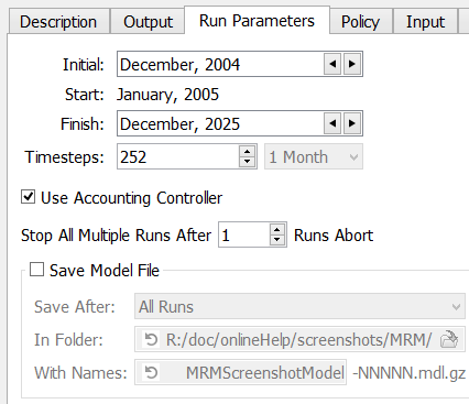
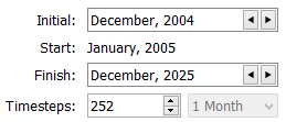
The Run Parameters tab describes the initial and end date of each concurrent run. The run parameters also show the timestep size, but timestep size is dependent on the model and can only be changed in the single run control dialog.
Note: The Initial and Finish timestep for a concurrent run can be different than what is shown in the single Run Control.
Use Accounting Controller
When Accounting is enabled, the Use Accounting Controller toggle is shown. This toggle allows you to decide if the multiple runs should use the accounting version of the controller or the non-accounting version. By default, the box is checked as that is the standard and most common behavior. De-select the option if you have accounting, but do not want to use an accounting controller for the multiple runs.
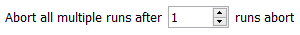
Control to Abort all Multiple Runs after Abort
Use the control to specify how many runs can abort before the total concurrent MRM is stopped. The default is 1, indicating all MRM runs will abort when any single run aborts. Increase this if you want to allow runs to abort but not stop all MRM runs.
During non-distributed concurrent MRM, diagnostic messages will indicate aborted runs. If the number of aborted runs does not cause the concurrent MRM to abort, the diagnostic message is shown as a green information message. If the number of aborted runs causes the concurrent MRM to abort, the diagnostic message is a red error message.
During distributed concurrent MRM, the number of runs which can abort before the concurrent MRM aborts is not per-simulation, it’s the total for all simulations. Consider a concurrent MRM which is configured to allow four traces to abort before the concurrent MRM aborts, and which is distributed across four simulations. Because the aborted trace limit is the total for all simulations, when the fourth trace aborts, the concurrent MRM will abort. This is independent of how the aborted traces are distributed among the simulations. If the user clicks the “show diagnostic messages” button, the messages identify which traces aborted.
See also Stop All Distributed Runs on Error for information on how distributed concurrent runs can be stopped when a given simulation stops.
Save Model File
The Run Parameters tab also allows you to configure to save the model after each run. This functionality is useful for debugging or if you want to see the resulting saved model file. To save the model after each run, select the Save Model File option and specify when to save the model, where and the name as follows:
– Save after: select one of the options:
• Successful Runs: This only saves the model for runs that completed successfully.
• Unsuccessful Runs: This saves the model for runs that abort.
• All Runs: Save the model for both successful and unsuccessful runs.
– In folder: select the folder in which to save the runs.
– With names: Specify the base model name. Each model will then be saved with that name and the suffix -NNNNN.mdl.gz. For example, ModelForDebugging-00001.mdl.gz, ModelForDebugging-00002.mdl.gz, etc.
Concurrent Runs tab
• The Concurrent Runs tab shows the number of runs that will be made.
– In most cases, the total number of runs should be the product of the number of rulesets, the number of input DMIs, and the number of index sequential runs:
#of MRM runs = #of Rulesets * #of Input DMIs * #of Index Seq Runs
– If the Pairs option for DMI/Index Sequential Mode has been selected on the Input tab, the total number of runs should equal the number of pairs of Input DMIs and Index Sequential runs. If the number of input DMIs does not match the number of Index Sequential runs, then the number of index sequential runs equals the total number of possible pairs, (i.e., the minimum of the number of input DMIs and the number of Index Sequential runs). (See the Index Sequential / DMI Mode section for more details.)
#of MRM runs = min(#of Input DMIs, #of Index Seq Runs)
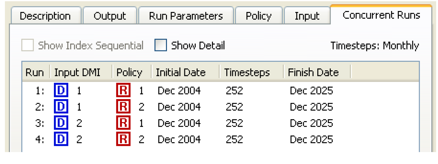
Figure 3.1 shows Concurrent Runs with 2 Input DMIs and 2 policy sets, no Index Sequential.
Figure 3.1
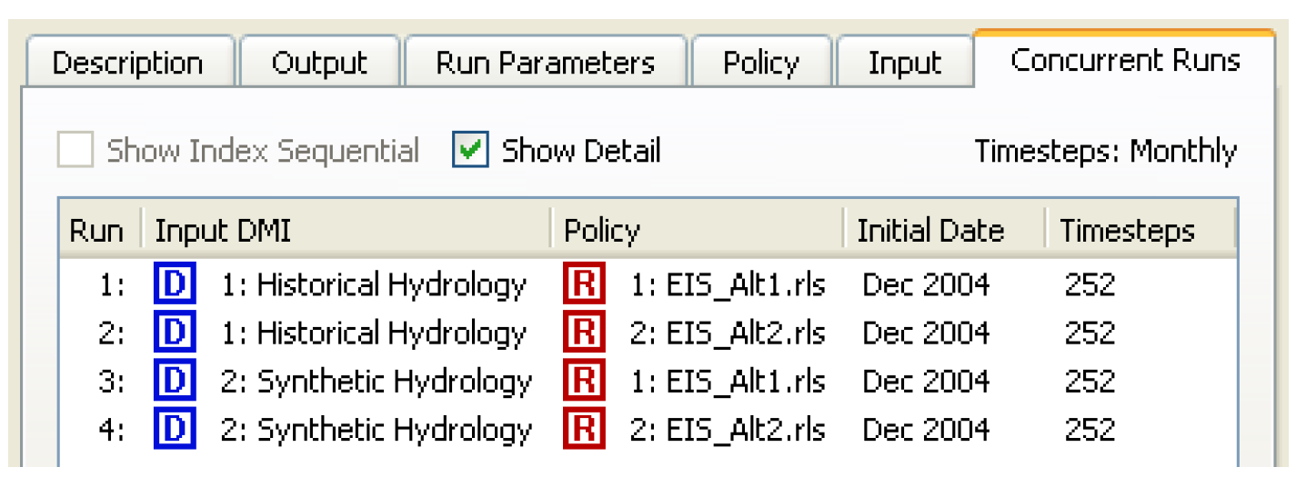
As shown in Figure 3.2, selecting the Show Details checkbox will show the names of the DMIs and policy sets.
Figure 3.2
Consecutive Runs
Consecutive runs are multiple runs where the time horizons are laid out consecutively. The end time of one run is the initial time of the next run. Timesteps do not vary among the different runs in a consecutive run.
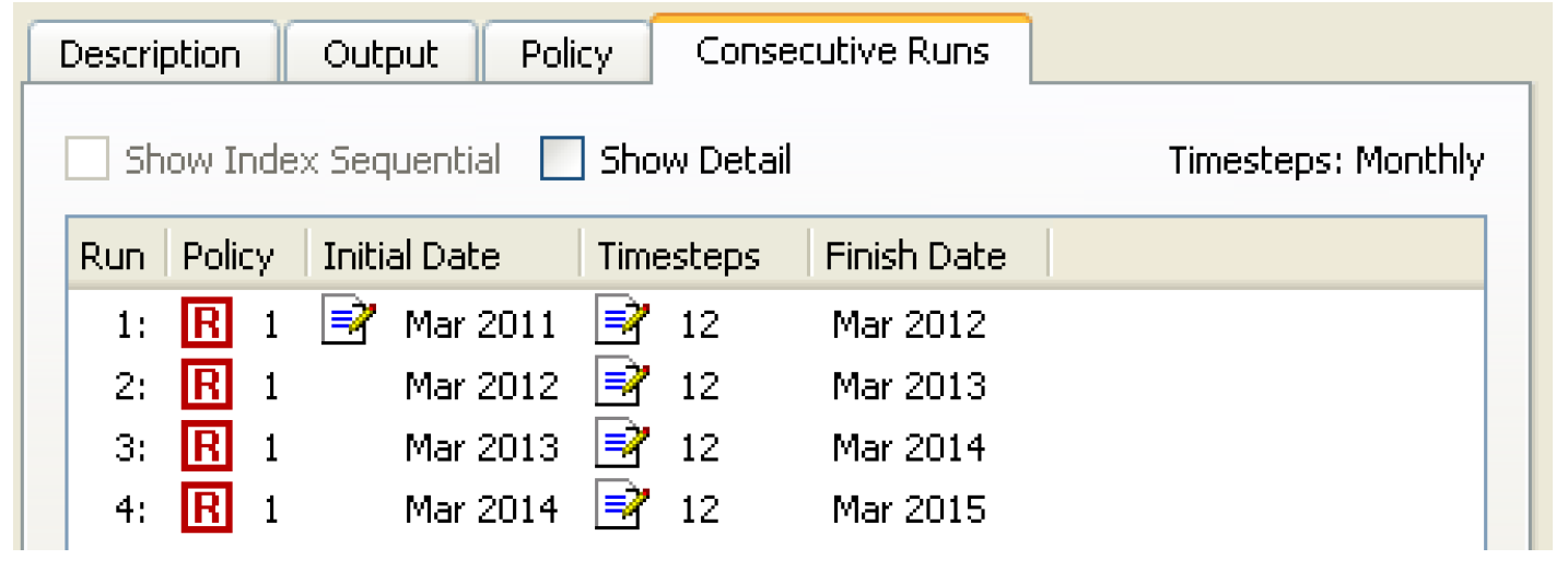
• On the Consecutive Runs tab, the Edit button indicates which fields in this dialog are editable.  If necessary, change the Initial Date for the consecutive runs. Do this by selecting the existing initial date and toggling the up/down arrows in the ensuing date-time spinner.
If necessary, change the Initial Date for the consecutive runs. Do this by selecting the existing initial date and toggling the up/down arrows in the ensuing date-time spinner. • Change the number of timesteps for the first consecutive run by selecting the existing number of timesteps and toggling the up/down arrows of the ensuing integer spinner. The Finish Date automatically updates.
• Append a new row for each desired additional consecutive run by selecting the Plus button. Or right-click below the existing consecutive run and selecting Append Row from the ensuing context menu. The Initial Date is automatically set to match the Finish Date of the previous consecutive run. In the Initial Date column, only the first consecutive run can be changed.
Or right-click below the existing consecutive run and selecting Append Row from the ensuing context menu. The Initial Date is automatically set to match the Finish Date of the previous consecutive run. In the Initial Date column, only the first consecutive run can be changed.• Change the number of timesteps for each individual run, if necessary. The default is for newly appended runs to have the same number of timesteps as the previous run.
• To remove a run, select the Minus button. This will always remove the last run. 
Iterative Runs
Iterative runs are multiple runs where MRM rules at the beginning and/or end of each run examine the state of the system and, if appropriate, set values for the subsequent simulation run. If no values are set or the maximum number of iterations occurs, then the simulation ends. As in concurrent runs, the time horizons, begin and end times and timestep length are all the same for all runs.
The iterative runs can use any of the controllers as specified in the single Run Control dialog: simulation (with or without accounting), rulebased (with or without accounting) or optimization. If the run is rulebased or optimization, the same RPL set or Goal set, respectively, is used in each iteration.
An iterative run executes as follows:
1. Initialize the iteration count.
2. Execute the Pre-MRM Run Rules, if specified.
Note: Pre-MRM Run Rules are similar to Initialization rules for each run; see Initialization Rules Set in RiverWare Policy Language (RPL).
3. Perform a single run.
4. Execute the Post-Run Rules, if specified.
5. If the Post-Run Rules return “no change”, that is they do not assign one or more new (different) values, the iteration is complete.
6. Otherwise, the iteration count is checked. If it equals the maximum number of iterations specified, then the iteration is complete also.
7. If the iteration is not complete, then increment the iteration count and return to Step 3..
When an MRM rule, either pre-run or post-run, sets a value on a slot, the value is given the i flag indicating that it is a “Iterative MRM” flag. Values with the iterative MRM flag are cleared at the beginning of an iterative MRM run but are not cleared between iterations of the MRM. This allows values set by the iterative MRM rules to persist between iterations but values are cleared at the beginning of the MRM run. In non-iterative MRM and single runs, values with an i flag are also cleared. You should be aware of this behavior if switching from iterative MRM to another mode.
Values set by the Iterative MRM “i” flag behave with output semantics. That is, they can be overwritten by any other value. In rulebased simulation, they are set when the controller is at priority zero, so values are given a priority of zero. Iterative MRM rules should only set values on data objects (typically integer indexed series slots as described at the end of this section), not simulation objects. Iterative MRM rules should be used to control the multiple runs; rulebased simulation rules within the run should be then used to set values on simulation slots that will actually be used in the run.
To configure an iterative run:
• Within the MRM Configuration dialog with the iterative mode, there is no Run Parameters tab. The iterative runs will begin at the start timestep of the model run. If users wish to change the model start timestep, this should be done in the single Run Control dialog.
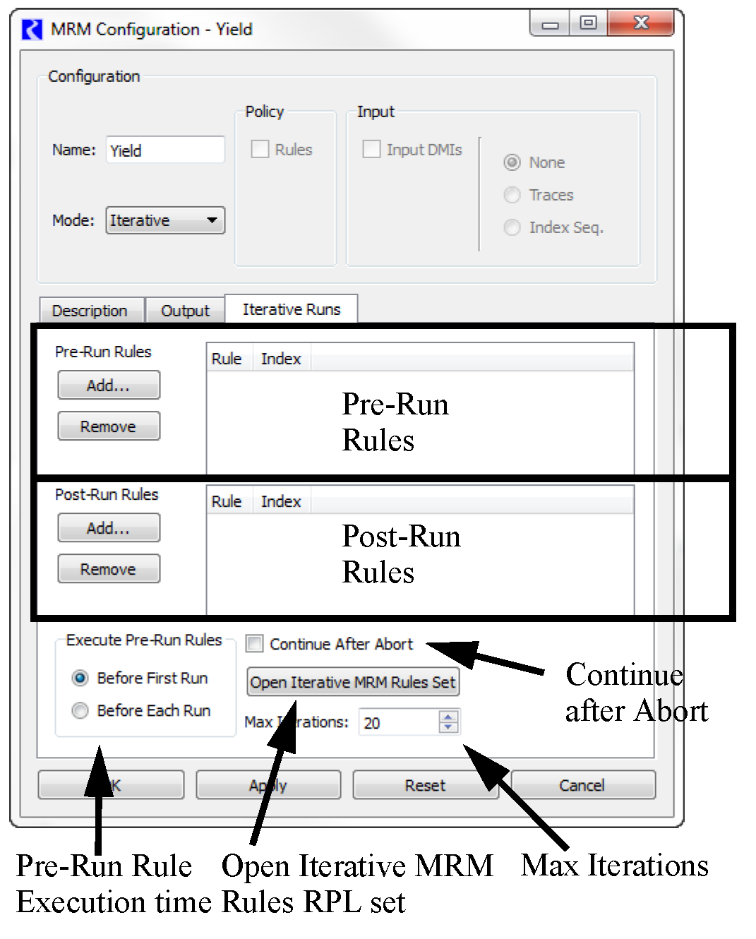
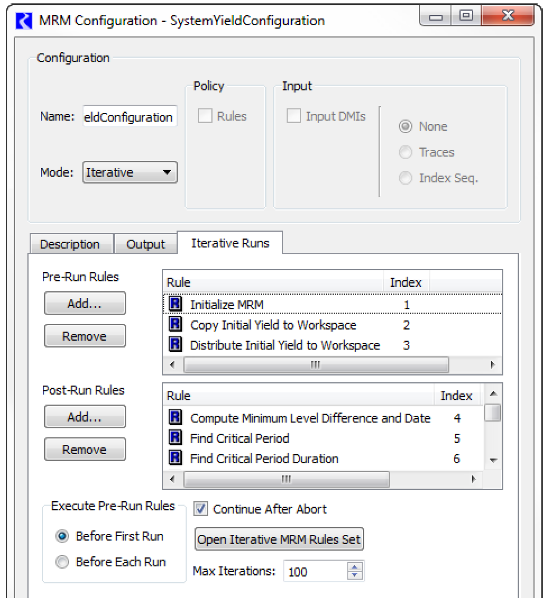
• On the Iterative Runs tab are the following significant areas: the Pre-MRM Run Rules, the Post-Run Rules, the Continue After Abort toggle, Pre-Run Rule Execution Time, the Open Iterative MRM Rules Set button, and the Max Iterations selector.
• Select Open Iterative MRM Rules Set button to open the Iterative MRM Rule set editor. This dialog operates very similarly to the standard RBS Ruleset Editor dialog. Create one (or more) Policy Group(s) and associated rules. The MRM Rules created are stored within the model file and may be available for use with any number of iterative MRM configurations. This set of rules can also be accessed from the workspace Policy, then Iterative MRM Rules Set.
• Once the MRM Rules have been built, return to the Iterative Runs tab of the MRM Configuration dialog. In this tab, the define which of the MRM rules should execute as part of the PreRun rules and which should execute after each iterative run, or both. These are defined in the appropriate areas using one of the following methods
– Use the Add and Remove buttons. Select the Add button to bring up the Rule Selector as shown in the following figure. This dialog shows the rule groups in a tree view. Expand the tree-view to show individual rule names, their Index and their On status. Select the checkbox to check the desired rules. Select Ok to accept and return to the configuration dialog.
– Drag and drop rules from the MRM Ruleset to the Pre-Run Rules area or Post-Run Rules area.
Note: The order of addition into the display does not affect the rule ordering; the order is strictly consistent with priorities defined in the MRM Rules.

• To view a rule directly from the Iterative Runs tab, double-click the rule’s name to open the Rule Editor.
• Use the Execute Pre-Run Rules buttons to specify when Pre-Run Rules are executed:
– Before First Run. This is the default. Choose this option to execute the Pre-Run Rules before the first single run only, but not before subsequent runs.
– Before Each Run. Choose this option to execute the Pre-Run Rules before each single run.
• Consider activating the Continue After Abort option. If you want the Post-Run Rules to execute and possibly the next iteration to begin after an iteration is prematurely aborted (for any reason), select the checkbox.
• Select the Max Iterations selector and adjust it using the up and down arrows or by typing a value in the field to define the maximum number of iterations to run. Figure 3.3 shows a fully configured Iterative Runs tab.
Figure 3.3
Note: The Post-Run Rules must make a significant change in values (for example, through a rule assignment or import of data through an input DMI) at the end of each run for the controller to make the next iteration. If the Post-Run Rules do not set any values, (possibly due to convergence) the controller will assume that the goal of the iterations has been achieved and stop.
Note: The MRM rules execute differently from the basic ruleset. When the MRM rules execute, each fires once and only once according to the execution order specified. There is no dependency functionality. In fact, they will all fire even if one of them aborts.
Integer indexed Series Slots work very well with Iterative MRM. Using these slots, you can store inputs, outputs, or intermediate results based on the index of the run. For example, after each iterative run, you could store the total volume of water released in an integer index slot in the row corresponding to the run index. At the end of the entire run, all of these volumes are stored and can be reviewed. The GetRunIndex predefined function can be used to get the index of the next iterative run. See Integer-indexed Series and Agg Series Slots in User Interface and GetRunIndex in RiverWare Policy Language (RPL) for details.
Policy
For concurrent and consecutive mode, a policy option can be specified for the runs. The policy setup of the configuration (None, Rules or Optimization) is selected from the Policy section of the MRM Configuration.
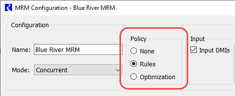
When None is selected, the multiple run uses the Simulation controller. When Rules or Optimization is selected, the Policy tab is added to the MRM Configuration. The Rules and Optimization options and the associated configuration on the Policy tab are covered in the following sections.
Note: The Policy options and the Policy tab are not applicable to Iterative MRM runs, but an iterative run can be a rulebased run or an optimization run where one ruleset or optimization goal set is used for all iterations. The ruleset or goal set must be loaded before the iterative run is started.
Rules
Selecting Rules for the policy option will enable the Rulebased Simulation controller when the multiple run is started. Rulebased multiple runs are runs in which there are one or more rulesets. You specify the ruleset to use for each run. Variations in rules can be a function of differences in content, priorities, or both.
• Select Rules under in the Policy section of the MRM Configuration and select the Policy tab.
• Specify whether to use the loaded ruleset or rulesets saved in files:
Figure 3.4 Screenshot of the MRM Policy tab
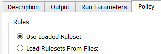
Use Loaded Ruleset
When specifying “Use Loaded Ruleset”, a single ruleset can be specified by loading it. The following behavior is used:
• For interactive MRM, the loaded ruleset and global function sets will be used. These sets can be loaded manually or can be saved in the model file and loaded when the model loads.
• For distributed MRM, the global function sets and the ruleset must be saved with the model file. If they are not, a validation error will occur at the beginning of the run.
For more information on saving sets in the model file, seeSave Location in RiverWare Policy Language (RPL).
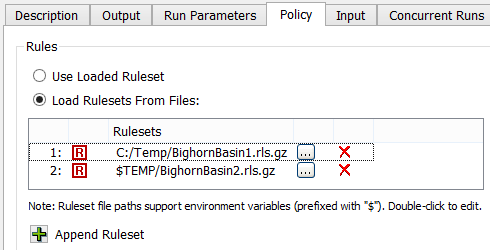
Load Rulesets from Files
When you specify to Load Ruleset from Files, you can specify one or more rulesets:
• Append a new row for each additional ruleset by selecting the Plus button at the bottom.
at the bottom.• Select the ruleset by selecting the File Chooser button  or double-click and type in the path name of the ruleset directly. This allows you to use environment variables in the path. Environment variables are prefixed with the “$”.
or double-click and type in the path name of the ruleset directly. This allows you to use environment variables in the path. Environment variables are prefixed with the “$”. • If necessary, remove a ruleset by selecting the Delete button  . There is no confirmation, but you can restore ruleset rows using the Reset button.
. There is no confirmation, but you can restore ruleset rows using the Reset button.In Figure 3.5, the first ruleset was specified by browsing to the C: drive, the second ruleset was specified by typing the path in directly and using the environment variable TEMP
Figure 3.5 Screenshot of the MRM Policy tab
Note: Multiple rulesets in a single MRM configuration are not supported if using Distributed Multiple Runs; see Distributed Concurrent Runs for details.
Optimization
Selecting Optimization for the policy option causes an optimization sequence to run for each individual run in the multiple run. On the Policy tab, you must configure the Run Sequence, Goal Sets and Post-Optimization Ruleset.
Note: Running optimization in RiverWare requires an optimization license. See Optimization License Required in Optimization for details.
Run Sequence and Optimization Restore Point
A single optimization run sequence is available: Simulation, Optimization and Post-Optimization RBS. This is the standard optimization sequence. The final outputs for each run are from the Post-Optimization RBS. See Standard Controller Sequence in Optimization for details on the optimization run sequence.
The Run Sequence configuration includes an option to Use Optimization Restore Point. In some cases all of the runs in a multiple run will be the same up to a certain priority in the goal set. For example, all runs may have the same input data, same high priority policy, and differ only in low priority objectives. The Restore Point feature allows each individual optimization run in the multiple run to begin from an advanced start, the last common goal, to reduce solution time by only solving the goals that differ. When using an Optimization Restore Point with MRM, the Restore Point must be created prior to the multiple run, in a separate optimization run. See Restore Point in Optimization for details on Optimization Restore Points.
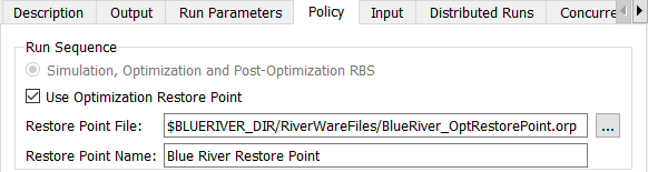
When specifying a Restore Point for MRM:
• Restore Point File: The Restore Point File must be specified for distributed MRM. For interactive MRM, the Restore Point File field is unused and is disabled. The Restore Point File must be created prior to starting the distributed multiple run. (See Export a Restore Point in Optimization for instructions to export an Optimization Restore Point to a file.) Each distributed multiple run will import the Restore Point from the file specified at the beginning of the multiple run. The Restore Point File can be specified by using the File Chooser button or by typing in the path name of the file directly. This allows you to use environment variables in the path. Environment variables are prefixed with the “$”.
or by typing in the path name of the file directly. This allows you to use environment variables in the path. Environment variables are prefixed with the “$”. • Restore Point Name: The Restore Point Name must be specified for distributed or interactive MRM.
– For distributed MRM, the Restore Point Name must match the name in the specified Restore Point File.
– For interactive MRM, the named Restore Point must be present in the Optimization Restore Point Manager when the multiple run is started. The Restore Point can either be imported from a file prior to the multiple run (see Import a Restore Point in Optimization or Import Optimization Restore Point in Automation Tools), or it can be created in by an interactive optimization run prior to the multiple run (see Create a Restore Point in Optimization).
Goal Sets
For the Goal Sets, you can choose either Use Loaded Goal Set or Load Goal Sets From Files.
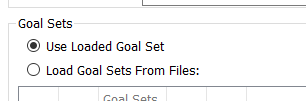
Use Loaded Goal Set
When you specify Use Loaded Goal Set, a single goal set can be used by loading it. The following behavior is used:
• For interactive MRM, the loaded goal set and global function sets will be used. These sets can be loaded manually or can be saved in the model file and loaded when the model loads.
• For distributed MRM, the global functions sets and the goal set must be saved with the model file. If they are not, a validation error will occur at the beginning of the run.
For more information on saving sets in the model file, seeSave Location in RiverWare Policy Language (RPL).
Load Goal Sets From Files
When you specify Load Goal Sets from Files, you can specify one or more goal sets:
• Append a new row for each additional goal set by selecting the Plus button at the bottom.
at the bottom.• Select the goal set by selecting the File Chooser button or double-click and type in the path name of the goal set directly. This allows you to use environment variables in the path. Environment variables are prefixed with the “$”.
or double-click and type in the path name of the goal set directly. This allows you to use environment variables in the path. Environment variables are prefixed with the “$”. • If necessary, remove a goal set by selecting the Delete button . There is no confirmation, but you can restore goal set rows using the Reset button.
. There is no confirmation, but you can restore goal set rows using the Reset button.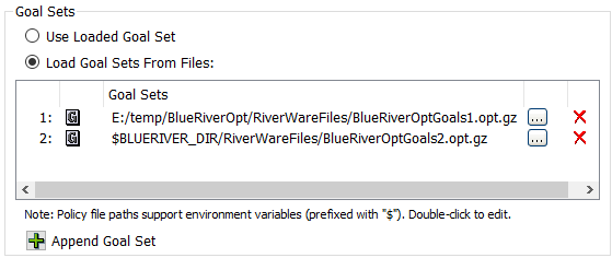
Note: Multiple optimization goal sets in a single MRM configuration are not supported if using Distributed Multiple Runs; see Distributed Concurrent Runs for details.
Post-Optimization Ruleset
A single post-optimization ruleset must be specified for the multiple run. You can chose either Use Loaded Ruleset or Load Ruleset From File.
• If Use Loaded Ruleset is selected, for interactive MRM, the set can be loaded manually or can be saved in the model file and loaded when the model loads. For distributed MRM, the set must be saved with the model file.
• If Load Ruleset From File is selected, the ruleset can be specified by selecting the File Chooser button or by typing in the path name of the ruleset directly. This allows you to use environment variables in the path. Environment variables are prefixed with the “$”.
or by typing in the path name of the ruleset directly. This allows you to use environment variables in the path. Environment variables are prefixed with the “$”. 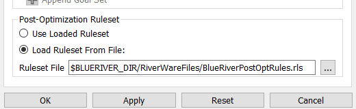
Input
Vary inputs for concurrent multiple runs by selecting options at the top of the MRM Configuration and then specifying configuration details on the Input tab.
Note: The Input section and tab are applicable and available only for Concurrent mode.
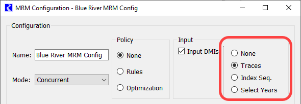
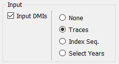
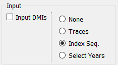
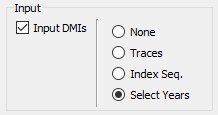
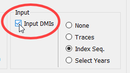
Four Input options are available.
• None
• Traces
• Index Sequential
• Select Years
If the Multiple Runs use an Input DMI, select the Input DMIs option in the Input section. See Input DMIs.
Optionally specify one Initialization DMI. See Initialization DMI.
If you wish to use ensembles with HDB datasets, select the HDB Input Ensembles checkbox. See HDB Ensembles for details.
None
When None is selected for the Input option, the number of runs in the multiple run is defined by the number of Input DMIs and their repeat counts. For example, if there are two Input DMIs specified, each with a repeat count of three, this would result in six runs (assuming a single policy specified on the Policy tab). If an Input DMI is repeated multiple times, it can make use of the Run Number or Trace Number to import the appropriate data for the specific run; see Input DMIs.
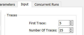
Traces
The Traces option allows you run a specific range of trace numbers.
1. Select Traces in the Input section of the MRM Configuration and select the Input tab.
2. Specify the First Trace and Number of Traces.
3. If using an Input DMI, the Repeat count for the DMI should be set to equal the Number of Traces. See Input DMIs.
Note: When using the Traces option, only a single Input DMI should be specified.
– Often a Trace Directory DMI is used with the Traces option. When this is the case, the trace number from the MRM configuration is used directly by the DMI to define the appropriate trace folder for the input data. See Trace Directory DMI in Data Management Interface (DMI).
– For a Control File-Executable DMI, the executable should reference the last command line parameter passed from RiverWare:
-STrace=traceNumber
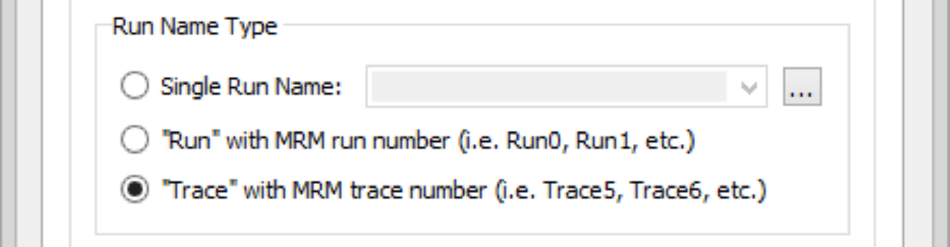
– For an Excel DMI, the Excel Dataset Run Name Type setting should use the Trace option; see Run Name Type in Data Management Interface (DMI).
Input DMIs are optional for the Traces mode. If no Input DMI is used, RPL logic in the model can utilize the GetTraceNumber predefined function to control the behavior of the logic for each trace.
Index Sequential
Index Sequential runs systematically shift inputs on series slots between runs. You specify the number of runs, the interval (number of timesteps) by which the input data is shifted from one run to the next, and an initial offset (number of timesteps) by which data is shifted for the first run. The slots with input data to be shifted are identified in a control file. This type of run is typically used to perturb (shift) historical hydrologic data in order to be able to conduct statistical analysis of the results.
For example, if an Index Sequential run is defined as the following:
• Original input time-series: Jan = 1, Feb = 2, Mar = 3, Apr = 4, May = 5, Jun = 6, Jul = 7, Aug = 8, Sep = 9
• Number of runs: 3
• Initial offset: 4 timesteps
• Interval: 1 timestep
then, the following sequence of runs occurs:
• Run 1: Jan = 5, Feb = 6, Mar = 7, Apr = 8, May = 9, Jun = 1, Jul = 2, Aug = 3, Sep = 4
• Run 2: Jan = 6, Feb = 7, Mar = 8, Apr = 9, May = 1, Jun = 2, Jul = 3, Aug = 4, Sep = 5
• Run 3: Jan = 7, Feb = 8, Mar = 9, Apr = 1, May = 2, Jun = 3, Jul = 4, Aug = 5, Sep = 6
If an Input DMI is used with Index Sequential, the DMI is executed once before the set of Index Sequential runs to import the input data. Then the data are rotated on the input slots for each run. (An exception to this is when the Pairs mode is used with Index Sequential; see Index Sequential Pairs Mode.)
To setup an Index-sequential run:
1. Select Index Sequential in the Input section of the MRM Configuration and select the Input tab.
2. Specify the Number of Runs, Initial Offset, and Interval by which the data is shifted from one run to the next.
3. Specify the units for the Initial Offset and Interval as Timesteps or Years.
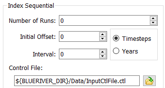
4. Specify the Control File by typing in the path directly or by using the file chooser to select it. Typing in the path and name directly allows for the use of environment variables. The control file specifies the slots that will be rotated for each run. It uses the same format as a control file for a Control File Executable DMI, but no file name or keyword value pairs are necessary. Typically, it is just the object and the slots that are specified. See Control File in Data Management Interface (DMI) for details.
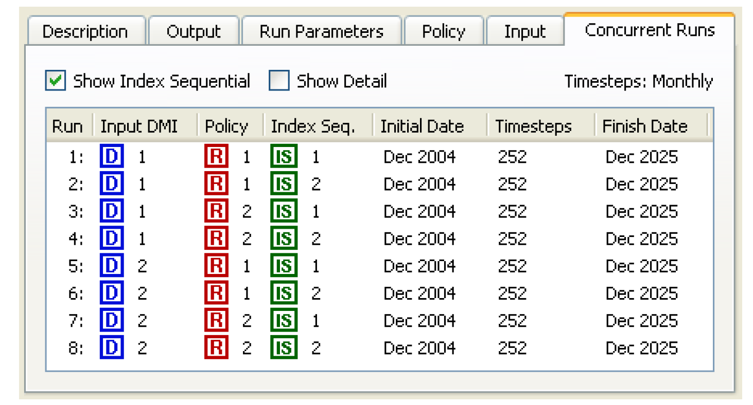
5. On the Concurrent Runs tab, the combinations of policy sets and Input DMIs are displayed for the index sequential runs.
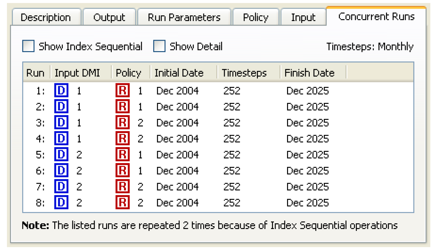
6. Select the Show Index Sequential option at the top of the Concurrent Runs tab to view each index sequential run listed individually.
Select Years
The Select Years option allows you to define the MRM traces based on selected historical years. The historical years are mapped to the run range. The number of traces simulated corresponds to the number of years selected.
When the Run Range is longer than one year, the selected year indicates the start year of the input for that trace. For example, if the Run Range is 5 years, May 20, 2021 to May 19, 2026, and a selected input year is 1972, the input data on the run timesteps (1 Day timestep size) May 20, 2021 to May 19, 2026 will come from May 20, 1972 to May 19, 1977.
If the selected year would cause the trace to extend past the end of the available data, the data will “wrap around” to the beginning of the dataset. For example, assume that data are available from January 1, 1903 to December 31, 2019, and 2017 is selected with the same five year Run Range as before. Inputs will come from May 20, 2017 to December 31, 2019 and then continue with January 1, 1903 to May 19, 1905.
The source data for each input slot should be in a single time series that spans the desired historical period.
Note: The Select Years option can be used only with constant timestep lengths, in other words, all timestep sizes of 1 Day and smaller. It cannot be used for 1 Month and 1 Year timestep sizes.
To use the Select Years option:
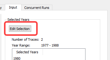
1. Select Years in the Input section of the MRM Configuration, and select the Input tab.
2. In the Selected Years section, choose the Edit Selection button.
3. In the resulting Select Years dialog box, specify the First Year and Last Year of the historical data that is available for import.
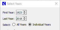
Note: The First Year and Last Year specified must have a complete year of data available in the data source, from January 1 to December 31, particularly if any of the traces from the selected years will “wrap around” to the beginning of the historical time series. The source data time series can extend past the First Year and Last Year specified, but only data within the specified First and Last Year will be used by the Input DMI.
4. Select whether to use All Years or Individual Years.
5. If Individual Years is selected, select which individual years to use. The check box at the top of the list can be used to quickly select or de-select all years. The Number of Traces will update to show how many years (traces) are currently selected.
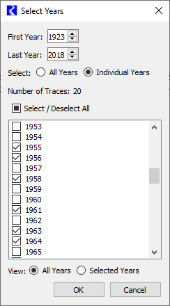
At the bottom of the Select Years dialog, there is an option to view All Years or Selected Years. This selection only affects which years are displayed in the dialog. It does not affect the year selection.
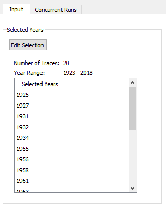
6. After completing the year selection, select OK. The Input tab will update to show the selected years and the number of traces, which corresponds to the number of selected years.
Note: The trace numbers reported in the output will correspond to the years selected. For example, if 1985 is one of the selected years, the trace that uses the data starting in 1985 will have the trace number 1985.
7. In the Input DMIs section, append an input DMI, and specify the DMI and Repeat count (see Input DMIs). The Repeat count should match the number of traces from the number of selected years.
Note: For the Select Years option, only a single Input DMI should be used.
The specified Input DMI should be either a Control File Executable DMI or a Database DMI, not a Trace Directory DMI. The DMI does not need to make use of trace information. The MRM will manage the traces by selecting the appropriate years of data from the full historical time series inputs. For an Excel DMI, the Single Run Name option should be used for the Run Name Type.

Note: When using the Select Years option, data will always be imported for the Start Timestep to Finish Timestep. For a Control File Executable DMI, if the start_timestep or end_timestep keywords are used in the control file, they will be ignored. For a Database DMI, if the Begin and End Timestep specifications are something other than Start Timestep and Finish Timestep, they will be ignored.
If the data import maps a leap year from the data source to a non-leap year in the run, the February 29 values from the data source will be omitted. If a non-leap year from the data source is mapped to a leap year in the run, the February 28 values from the data source will be duplicated for February 29 in the run except for the case that the Start Timestep of the run is February 29, in which case the March 1 values from the data source will be duplicated for February 29.
Initialization DMI
You can optionally specify a single DMI or DMI group that is invoked once at the beginning of the multiple run. An Initialization DMI would be used to import data that is common to all runs in the multiple run.
Select the Initialization DMI option to show the entry field. Type in the name of an existing DMI or use the  button to select an the DMI or DMI group.
button to select an the DMI or DMI group. 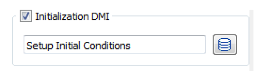
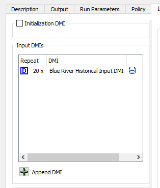
Input DMIs
Input DMIs execute at the beginning of each individual run in the multiple run and import the data specific to that run for a specified set of slots. Input DMIs can be used with any of the four Input options. They are required for the None and Select Years options. The Input DMIs must be previously defined in the RiverWare DMI interface; see DMI User Interface in Data Management Interface (DMI).
1. Select the Input DMIs option at the top of the MRM configuration.
When the Input DMIs option is selected, the Input DMIs section becomes active on the Input tab.
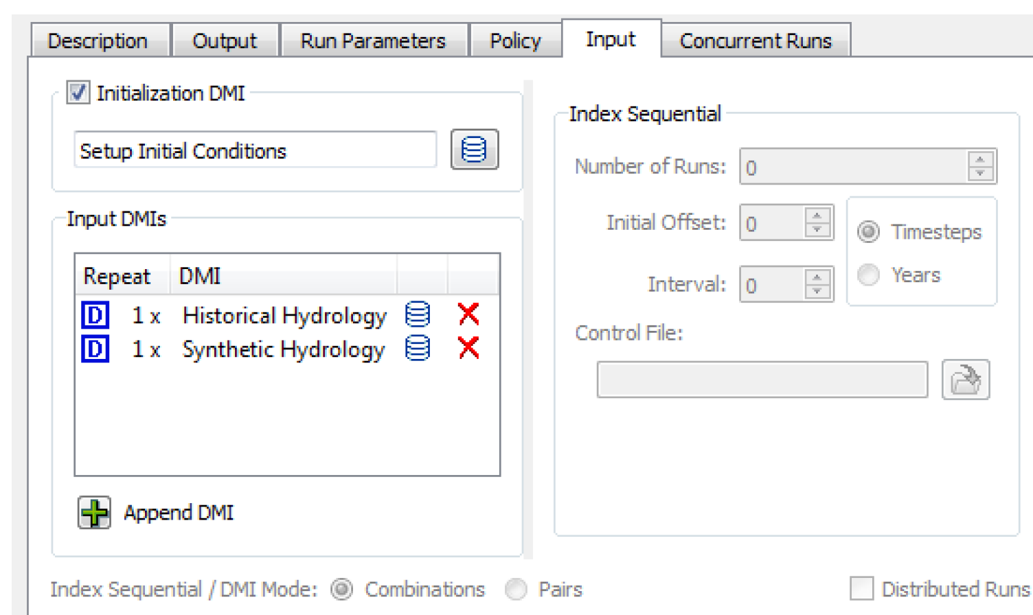
2. Append a new DMI by selecting the Plus button for Append DMI at the bottom.
for Append DMI at the bottom.3. Select the input DMI (or DMI group) by selecting the DMI icon  and then choosing the previously configured DMI from the list.
and then choosing the previously configured DMI from the list.4. If the DMI will be called more than one time, change the number in the Repeat column by double-clicking the cell and using the up/down arrows. DMIs might need to be called more than once with multiple runs that execute multiple traces using the same DMI. In this situation, the DMI needs to be configured to make use of the trace number.
– For a Control File-Executable DMI, the executable should reference the last command line parameter passed from RiverWare:
-STrace=traceNumber
– For a Trace Directory DMI, the trace number will be used directly to determine which trace folder to access. See Trace Directory DMI in Data Management Interface (DMI).
– For an Excel DMI, the Excel Dataset Run Name Type setting should use either the Run or Trace option; see Run Name Type in Data Management Interface (DMI). The Run numbers are always 0 through the number of runs in the multiple run. The Trace numbers can be any positive integer, depending on how the inputs are configured.
Warning: The “Run” option cannot be used with distributed MRM because in each distributed RiverWare process, the run numbers start at zero. A DMI error will be issued in this case.
Warning: DSS DMIs are not compatible with MRM as there is no way to change the part information for a particular run in an MRM.
Note: Each run in the multiple run invokes a single DMI or DMI group at the beginning of the run. For example, if the MRM configuration includes DMI 1 and DMI 2, each with a Repeat count of 3, this corresponds to six runs. The first three runs will use DMI 1. The next three runs will use DMI 2 (as opposed to three runs that invoke both DMIs at the beginning of each run). If it is necessary to invoke multiple input DMIs at the beginning of each run, they should be included in a DMI group, and the DMI group should be selected in the Input DMIs section of the MRM configuration. See DMI Groups in Data Management Interface (DMI).
If you wish to use Ensembles with HDB datasets, select the HDB Input Ensembles checkbox. See HDB Ensembles for details.
Concurrent Runs
By default, the runs that are made in concurrent MRM are a multiplicative combination of inputs. This set is called Concurrent Runs. Concurrent runs are defined as the Cartesian product of all the involved base-type runs. For example, a, MRM configuration consisting of two rulesets and four Input DMIs, results in eight model runs.
The order in which individual runs within a multiple run are executed is determined by the precedence level of each mode. Order of precedence (from highest (1) to lowest (3)) is as follows:
1. Input DMIs,
2. Policies (rulesets or optimization goal sets), and
3. Index-Sequential
Elements of lower precedence iterate before elements of higher precedence. For example, in case of a concurrent multiple run containing two Input DMIs and two rulesets, the following sequence of four runs is made:
1. Input DMI 1 & Ruleset 1.
2. Input DMI 1 & Ruleset 2.
3. Input DMI 2 & Ruleset 1.
4. Input DMI 2 & Ruleset 2.
Thus, the default combinations mode results in the total number of runs equal to the product of the number of policy sets, the number of input DMIs, and the number of index sequential runs:
#of MRM runs = #of Policy Sets * #of Input DMIs * #of Index Seq Runs
The list of resulting runs can be viewed on the Concurrent Runs tab.
Index Sequential Pairs Mode
In very specific circumstances, it is possible to alter the mode of how many MRM runs result from the combination of input DMIs, policy sets, and Index Sequential runs. If Index Sequential has been selected and there are as many (or more) Input DMIs as Index Sequential runs and there are zero or one rulesets selected, then it is possible to choose either Combinations or Pairs in the Index Sequential / DMI Mode selection.
The Pairs mode results in the total number of runs equaling the number of pairs of Input DMIs and Index Sequential runs. If the number of input DMIs does not match the number of Index Sequential runs, then the number of index sequential runs equals the total number of possible pairs, (i.e., the minimum of the number of input DMIs and the number of Index Sequential runs). The Pairs mode is necessary to run the CRSS Lite model.
# of MRM runs = min(# of Input DMIs, # of Index Seq Runs)
When the pairs mode is specified, the runs can be distributed to multiple processors. See Distributed Concurrent Runs for details.
HDB Ensembles
An ensemble contains a set of traces where each trace represents the data for one run of the multiple run. An ensemble of trace data can function as input to the runs of a multiple run or can represent output from a multiple run. MRM provides configuration for running ensembles specific to Database DMIs with HDB Datasets. (See HDB Datasets in Data Management Interface (DMI) for information on HDB Database DMIs.) An HDB Ensemble can have metadata that describes the overall ensemble and metadata that describes each of the individual traces.
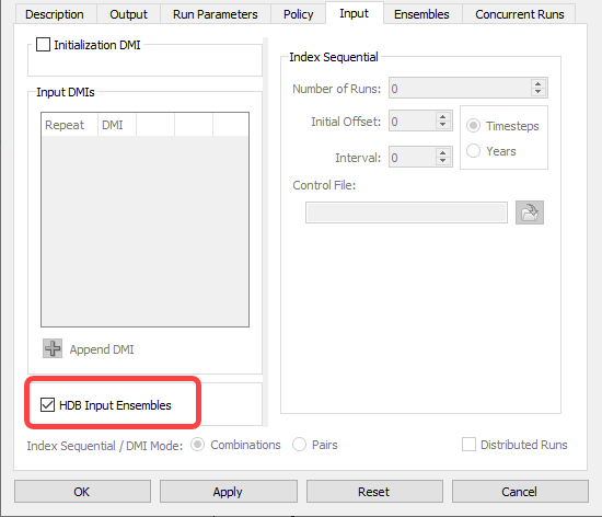
HDB Ensemble Configuration
To utilize HDB Ensembles, on the Input tab of the MRM configuration, select the HDB Input Ensemble option at the bottom left of the Input tab. This will disable Input DMIs, Traces, and Index Sequential functionality as the ensembles will determine the number of runs in the multiple run.
When you select HDB Input Ensembles, an Ensemble tab is added to the MRM Configuration. The Ensemble tab is where input and output ensembles are specified.
On the Ensembles tab select the Plus in the Input Ensembles frame to open a list of input DMIs defined in the model. Only valid input DMIs with HDB datasets configured with ensembles can be added.
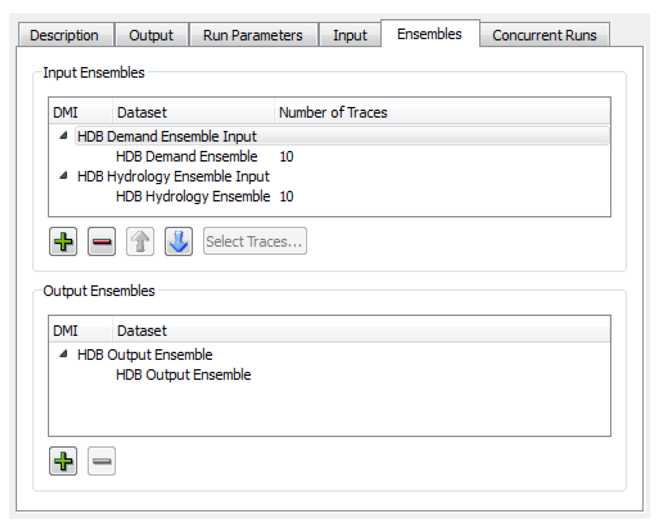
Input DMIs will be executed in the order shown. This allows you to configure how data is loaded if the same slots are used in multiple input DMIs (the last one in wins). Use the up and down arrow buttons to reorder the selected DMI.
When a DMI is added as an input ensemble, it defaults to using all of the traces defined in the ensemble. The Number of Traces column shows the number of traces for each DMI. When an item having traces is selected in the list, the Select Traces button is enabled. Select this button to open a dialog showing all of the traces for the ensemble, and choose a subset of traces as desired.
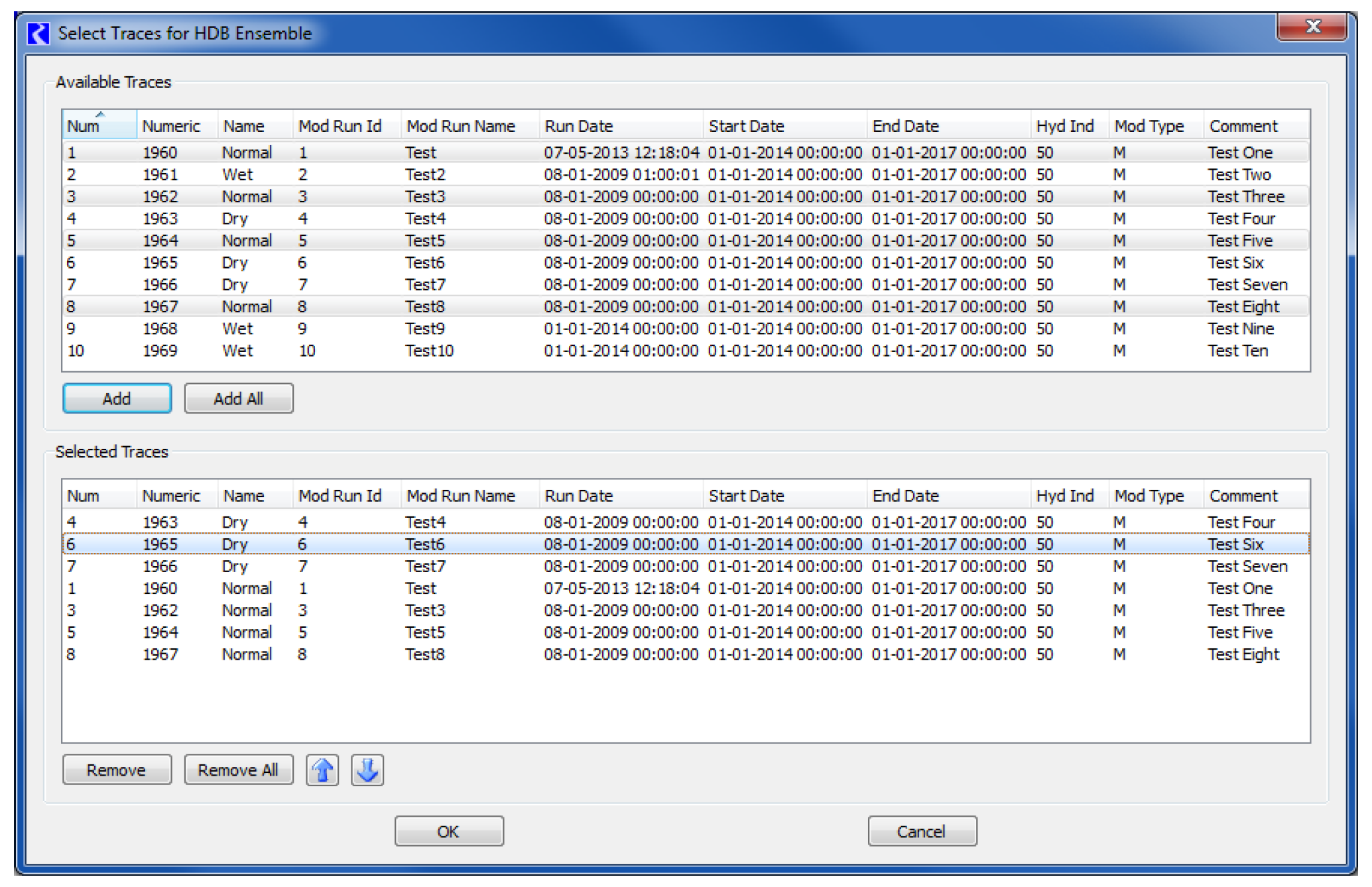
All available traces are presented in the upper list. When added using the Add or Add All buttons, they are copied to the lower list showing the selected traces. Traces can be removed from the selected list with the Remove or Remove All buttons. The selected traces can be ordered using the up and down arrow buttons. With these controls, a subset of traces in the ensemble can be chosen and used in any order as input to the multiple run. When applied with the OK button, the number of selected traces will appear in the Number of Traces column in the Input Ensembles frame of the Ensembles tab.
The number of traces for input ensembles must match across all of the input ensembles because the number of traces input to the multiple run will determine the number of runs. If an MRM configuration with differing numbers of input ensemble traces is applied or a run is started, an error message is generated.
HDB ensemble datasets have an option to defer picking an ensemble for the dataset until the MRM run is started. See HDB Table Type—Ensembles in Data Management Interface (DMI) for details. In this case, the Number of Traces column will show a zero, and using the Select Traces button will return a message that the ensemble will not be selected until MRM start. Where datasets of this type are used in input ensembles, the number of runs in the multiple run cannot be determined until the MRM run is started, so the Concurrent Runs tab of the MRM configuration dialog will be empty. Uniformity of number of traces across input ensembles is checked after ensembles are selected at the start of the MRM run.
DMIs to use as output ensembles are added and removed with the plus and minus buttons in the Output Ensembles frame of the Ensembles tab. Unlike input ensembles, the order of output ensembles does not matter, so there are no ordering controls in this frame. All existing data and metadata in output ensembles for a multiple run are cleared at the beginning of the multiple run. At the end of each run in the multiple run, the data specified in output ensemble DMIs are written to the trace of the output ensemble that corresponds to that run. An output ensemble must have at least as many traces as the number of runs in the multiple run so that all of the run data can be written. If an HDB dataset configured to select the ensemble at MRM start is used in an output ensemble, its number of traces is checked after the ensemble is selected.
HDB Ensemble Metadata
An HDB Ensemble can have metadata that describes the ensemble as well as metadata that describes each trace in the ensemble. Metadata is represented in RiverWare as Keyword/value pairs, such as “comment”/”Climate Change Hydrology”. An important functionality of HDBEnsembles with MRM is that the ensemble and trace metadata from input ensembles are combined and copied over to output ensembles.
For ensemble metadata, values for the “domain”, or “comment” keywords from input ensembles are concatenated with semicolons and written as values for these keywords to output ensembles. For example, if there were two input ensembles, one with a comment “Historic Hydrology” and the other with a comment “High Projected Demand”, an output ensemble would be given the comment keyword value of “Historic Hydrology;High Projected Demand”. Values for other ensemble metadata keywords are not concatenated. If values for these other keywords differ among input ensembles, the keyword value from the first ensemble is copied to the output ensemble and a warning issued that values for this keyword differ among the input ensembles.
For trace metadata, values for the “name” keyword for multiple input ensemble traces will be concatenated with semicolons and written as the value for the “name” keyword to an output trace. Values for other trace metadata keywords are not concatenated. If values for these other keywords differ among multiple input ensemble traces, the keyword value from the trace of the first ensemble will be copied to an output ensemble trace and a warning issued that values for this keyword differ among the input ensemble traces.
See HDB Table Type—Ensembles in Data Management Interface (DMI) for details on HDB ensembles and metadata.
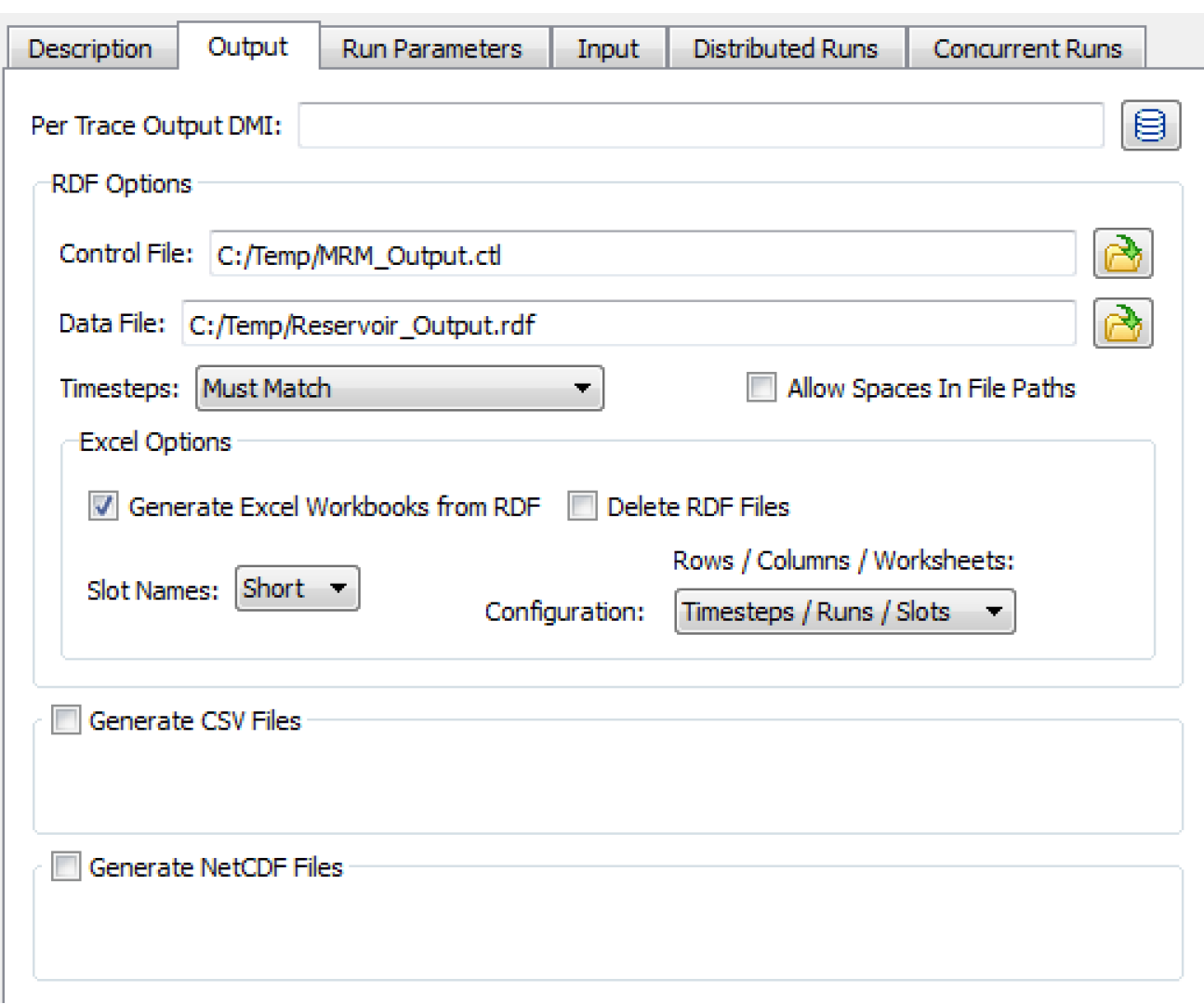
Output
During a multiple run, output can go to an output DMI and/or one or more RiverWare Data Format (RDF) text files. Options are also available to send output to CSV files or NetCDF files. Select the Output tab of the Multiple Run Editor. The following figure and subsequent sections show the configuration options:
Per Trace Output DMI
The optional Per Trace Output DMI field allows selecting or entering an output DMI or a group of output DMIs that will be run after each single run of the multiple run. HDB ensemble datasets cannot be used in these DMIs, but rather must be used in the MRM ensemble configuration; see HDB Ensemble Configuration for details.
The DMIs must be previously configured in the DMI Manager in RiverWare. The executable that is configured for the DMI can reference the trace number of the run that is outputting by referencing the last command line parameter passed from RiverWare:
-STrace=traceNumber
RDF Options
Send MRM outputs to RiverWare Data Format text files. These files can be automatically converted to Excel files or processed using outside tools.
Tip: See Ensemble Data Tool for more information on viewing and analyzing the results of an MRM run using the Ensemble Data Tool.
Configurations for RDF output from MRM include the following:
Control File
Type or use the File Chooser button to select a complete file path into the required control file field. The control file is used to specify which slots are output after each MRM run. The control file may contain “file =” specifiers for any line entries in the file. This causes data associated with those lines to go to the specified RDF output file. In the example control file below, if “fileName” is the same for each slot, then the output will go to a single RDF file; varying file names will send the output to multiple RDF files.
MountainStorage.Inflow: file=fileName
MountainStorage.Outflow: file=fileName
MountainStorage.Storage: file=fileName file=fileName2
MountainStorage.Pool Elevation: file=filename3 start_timestep=”Start Timestep - 1 timestep”
File Specification
You can optionally specify multiple files for a single slot as in the third line above. Also, slots with a timestep different than the model’s timestep can be output using the same syntax.
In the control file, there are four ways to specify where the data files are created:
• Hard code the path: file=C:/DMI/Data/ResA.Inflow
• Use an environment variable: file=$(DMI_DATA)/ResA.Inflow
• Use '~': file=~/ResA.Inflow where '~' is replaced with $RIVERWARE_DMI_DIR/<DMI name>
• If the filename is not specified, the output file will be created in the directory in which RiverWare resides.
The second option is recommended as it is more transparent than '~” but still allows the model to be moved from machine to machine by setting the environment variable to the appropriate value on each machine.
Start and End Timestep Specification
Within the control file, optionally specify the start_timestep and end_timestep in the control file for each slot specification. If not specified, the MRM run’s start and finish timestep will be used.
Both of these keywords allow you to also specify the timestep symbolically using RPL syntax. For example, the following are valid entries:
• start_timestep=“24:00 November Max DayOfMonth, 1996”
• start_timestep=”Start Timestep - 1 timestep”
• start_timestep=“Start Month Start DayOfMonth, Start Year - 2 days”
• end_timestep=“24:00 3/1/2021”
• end_timestep=”Finish Timestep + 10 days”
See DATETIME in RiverWare Policy Language (RPL) for details on datetimes. Basically, any fully specified datetime can be used. No @ symbol is necessary but quotes are necessary when specifying datetimes that contain spaces.
Note: Current timestep is not supported in this context.
Caution: A particular RDF file must have the same date range for all slots. Thus, if you send data for the MRM Run Range to one RDF file, you cannot also send pre-run data to that same RDF file. You would need to have a separate RDF file for pre-run data. If you tried to send it to the same RDF file, it would give a warning and then skip slots that do not match the given range. The first slot written to an RDF file determines its range.
Resolving Conflicts in Slot Entries
It is possible that more than one control file entry line will represent a slot on the workspace. For example:
LevelPowerReservoir.Outflow: file=AllResData.rdf
BigRes.Outflow: file=AllResData.rdf
In this case, the more exact entry (the second one) will take precedence and the Outflow will be written to AllResData.rdf. If the slot, time interval and file specification resolve to the same value for one or more slot entry lines, the more exact specification takes precedence and is used in the metacontrol file and the RDF file.
The control file entries are considered different and the values will be written separately to the specified RDF files whenever the control file entry lines have:
- different slots,
- different time intervals, or
- different RDF file specifications
If any of these three are different, there is no need to determine the more exact entry. Instead, the slot data is written out as a separate entry to the metacontrol file and then to the RDF file. For example:
LevelPowerReservoir.Outflow: file=AllResData.rdf
BigRes.Outflow: file=BigResData.rdf
Although the slot specification would be the same for BigRes.Outflow (as above), the files are different, so the slot values are written to both AllResData.rdf and BigResData.rdf.
With this approach, it is possible that a slot could be written multiple times to the same RDF file.
Data File
Optionally type or use the File Chooser button to select a complete file path into the Data File field. This file is used as the RDF output file for any lines in the control file that do not have an explicit file specifier. If the data file field is used and there are no “file=” specifiers in the control file, then all output will go to this single data file.
Timesteps
Specify whether RDF output files may contains slots whose timestep sizes differ. There are three choices:
• Must Match. All slots written to an RDF file must have the same timestep size. Slots whose timesteps differ from the file’s timestep are skipped. (The file’s timestep is determined by the first slot MRM associates with the file.) You are warned about slots being skipped, and asked whether to continue the MRM run.
• Use Smallest. Slots written to an RDF file may have different timestep sizes, with the output written using the smallest timestep.For example, if slots with 1 Month and 1 Year timesteps are written to an RDF file, monthly values will be written and the 1 Year slots will write 11 NaN followed by a value.
• Use Largest. Slots written to an RDF file may have different timestep sizes, with the output written using the largest timestep. For example, if slots with 1 Month and 1 Year timesteps are written to an RDF file, yearly values will be written and the 1 Month slots will write December values.
Allow Spaces in File Paths
The Allow Spaces in File Paths allows file paths that have spaces. Without this box checked, the RDF control file paths would replace spaces in with ‘_’.
Excel Options
Select Generate Excel Workbooks from RDF to create Excel files from all of the RDF output files after all runs have completed.
Select Delete RDF Files to delete all RDF files after the Excel files are created. (The separate RdfToExcelExecutable program contains the same functionality for creating Excel files from RDF files and can be used outside of RiverWare to process RDF files from an MRM run.)
Select a Configuration from the menu to control how timestep, slot, and run data from RiverWare are mapped onto the Excel dimensions of rows, columns, and worksheets.
Select an option from the Slot Names menu to specify how slot names are written into the Excel workbook. Options are as
• Index: (Slot0, Slot1, etc.)
• Short: Automatically shortened names (lower case vowels removed)
• Full: Full slot names (limited to 31 characters for worksheet names, which is the limit for Excel)
CSV Files
CSV files can be generated from the MRM run outputs. The CSV files are formatted for direct use within Tableau data visualization software. The configuration allows for the selection of various pieces of information to be used as dimensions in Tableau. The CSV output is essentially a table with the columns delimited by commas.
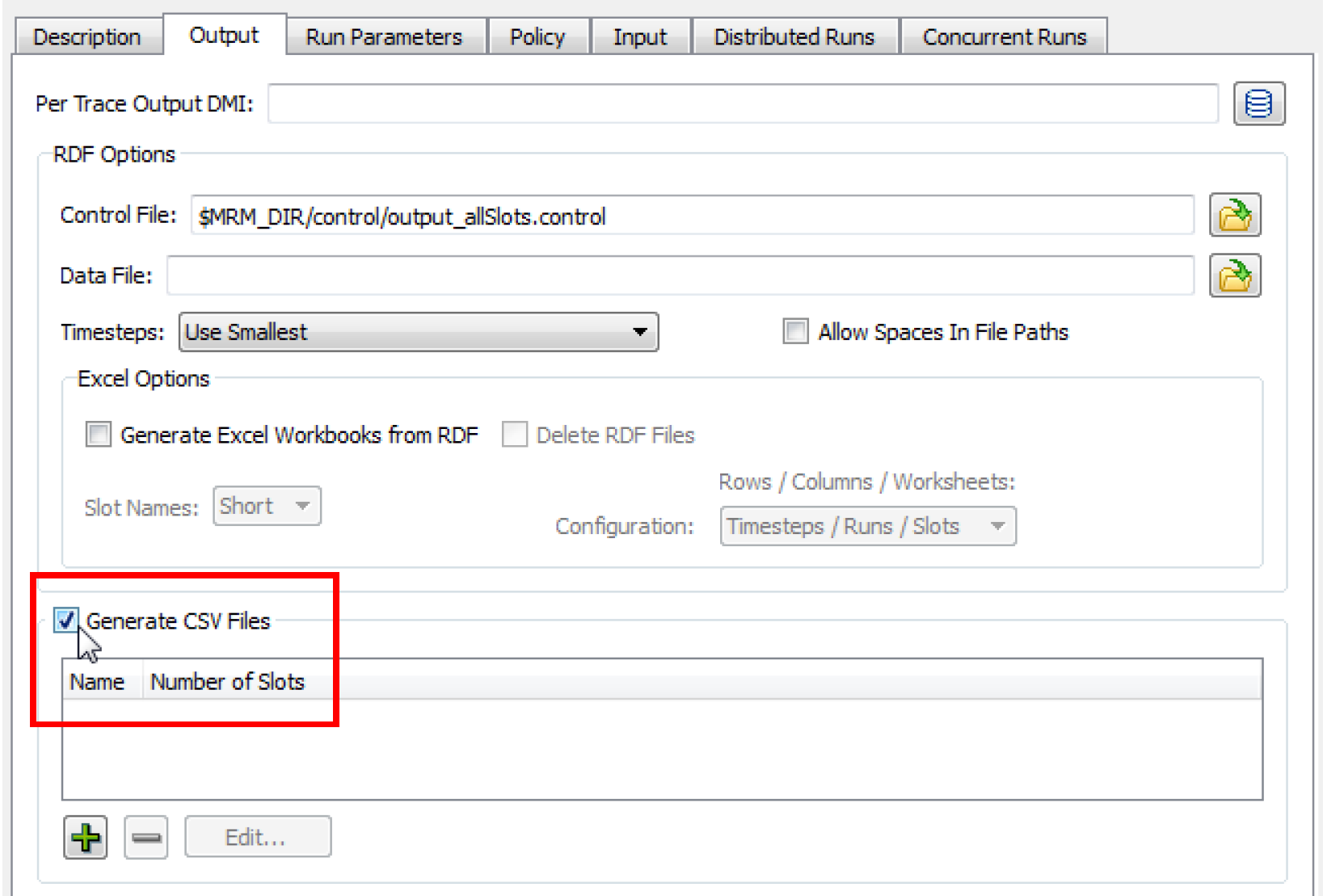
1. Near the bottom of the Output tab in the MRM configuration dialog, select the checkbox for Generate CSV Files.
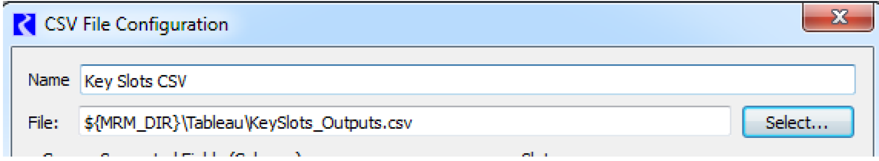
2. Select the Plus sign to add a new CSV output file. Then select Edit to configure its contents. This will open the CSV File Configuration dialog.
3. The CSV can then be given a name to display in the list in the MRM configuration.
4. In the File field, either select a CSV file to which the new outputs should be written by selecting the Select button, or type in a complete file path. Environment variables can be used in the file path preceded by a “$”.
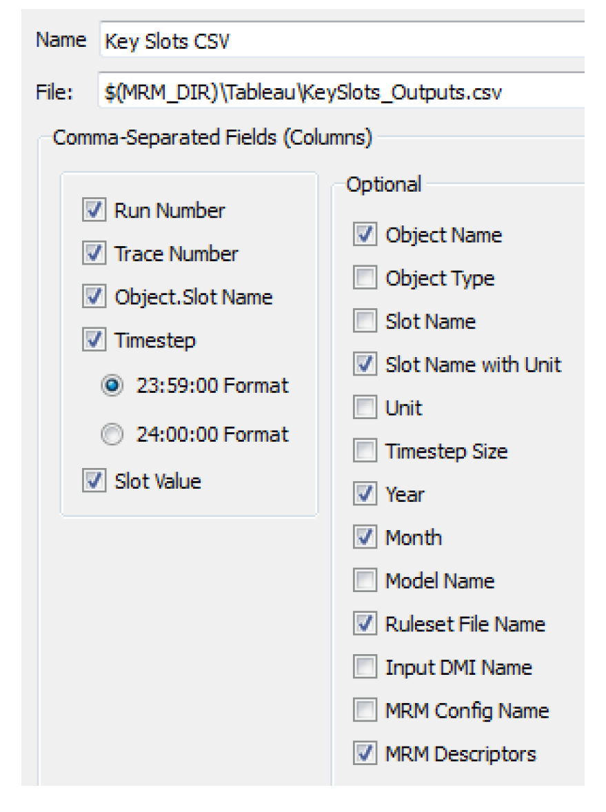
5. Next, select which pieces of additional information should be included as columns in the output table by selecting or clearing the checkbox by each optional element. Figure 3.6 shows the list of available elements. The CSV output file will contain a column for each item selected. The text shown in the CSV File Configuration dialog will be used as the column header. The Slot Value column is the only column that will contain true “output” data from the MRM run. The Slot Value will be considered a “measure” within Tableau. The remaining columns contain information associated with each Slot Value and will be considered dimensions within Tableau.
Figure 3.6
Note: In the context of Distributed Multiple Runs the Run Number corresponds to the run number on the individual processor. Thus if there are eight runs distributed to four processors (two each), all rows in the resulting CSV file will show a Run Number of either 1 or 2.
6. Then add slots to the CSV output by selecting Plus sign below the Slots panel. This will open a slot selector dialog, which can be used to add the desired slots. A slot can be removed from the selection by selecting it in the list to highlight it, then selecting the Minus sign.
7. After configuring the CSV output, select OK in the CSV File Configuration dialog, and select Apply or OK in the MRM Configuration dialog to apply the changes.
During the MRM run, RiverWare will write the outputs to the specified CSV file. The file will contain one row for each selected slot at each timestep for each run. For each row, the columns will be filled in appropriately by RiverWare based in the selected dimensions. Figure 3.7 shows part of a sample CSV output file (viewed in Microsoft Excel).
Figure 3.7
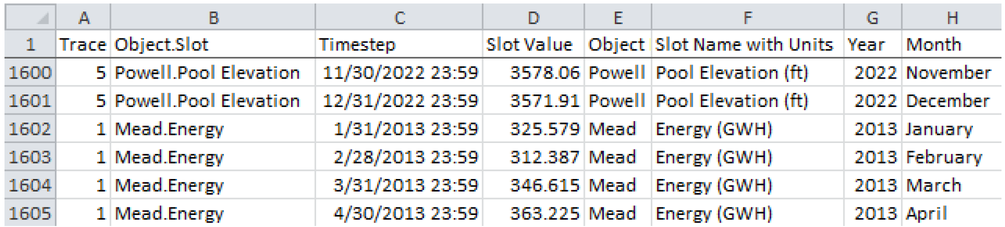
RiverWare uses end of timestep format for all datetime references. Thus for a 1 Month timestep, July 2014 would be fully specified as 7/31/2014 24:00. Tableau and Excel do not have a concept of 24:00 as a time but would instead use 8/1/2014 00:00 for the same point in time. Therefore with the proper timestep option selected in the dialog, one minute is subtracted from all timestep values (e.g. 7/31/2014 23:59) to assure that they appear with the appropriate day and month references in Excel and Tableau.
Note: If the specified CSV file already exists, the CSV output from the new MRM run will overwrite the existing CSV file. It will not append data to the existing file.
NetCDF Files
Network Common Data Format (netCDF) files can be generated from the MRM run outputs. The configuration allows for the selection of various pieces of information to be used as global attributes and slot (variable) attributes. Time and Traces are treated as dimensions.
Note: RiverWare will write the file in the netCDF-3 format, with one unlimited dimension (time). The output does not use any of the features available in netCDF-4 and testing has shown that netCDF-3 provides a much smaller file size than using netCDF-4.
1. Near the bottom of the Output tab in the MRM configuration dialog, select the checkbox for Generate NetCDF Files.
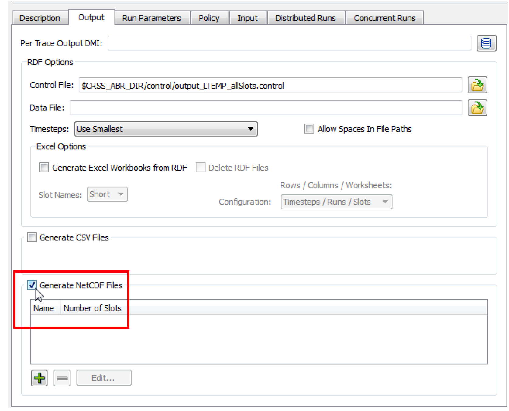
2. Select the Plus sign to add a new netCDF output file. Then select Edit to configure its contents. This will open the NetCDF File Configuration dialog.
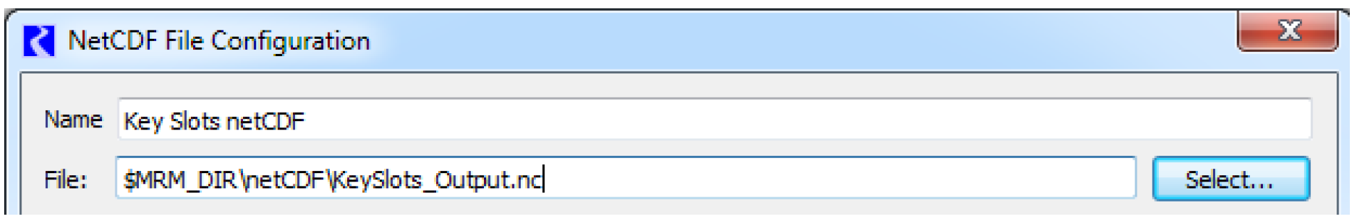
3. The netCDF file can then be given a name to display in the list in the MRM configuration.
4. In the File field, either select a netCDF file to which the new outputs should be written by selecting the Select button, or type in a complete file path. Environment variables can be used in the file path preceded by a “$”.
5. Next, optionally select global attributes and slot attributes to be included with the outputs by selecting or clearing the checkbox by each element.
Note: Time (timestep) and Traces (Trace Number) will automatically be used as dimensions in the netCDF output.
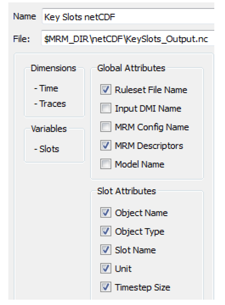
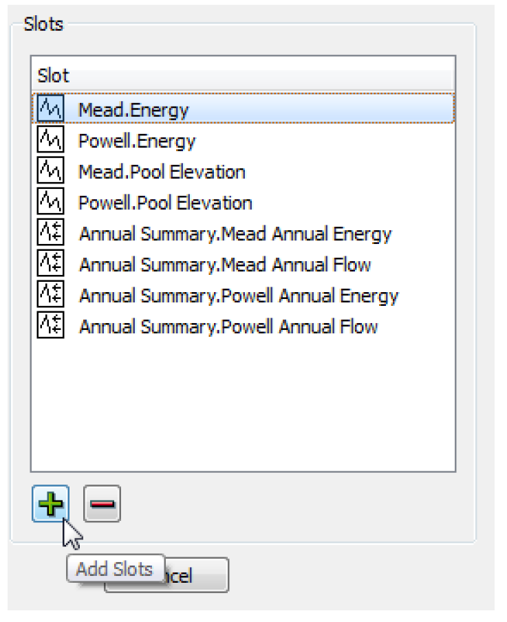
6. Then add slots to the netCDF output by selecting the Plus sign below the Slots panel. This will open a slot selector dialog, which can be used to add the desired slots. A slot can be removed from the selection by selecting it in the list to highlight it, then selecting the Minus sign. The Object.Slot name will be used as the variable name in the netCDF file.
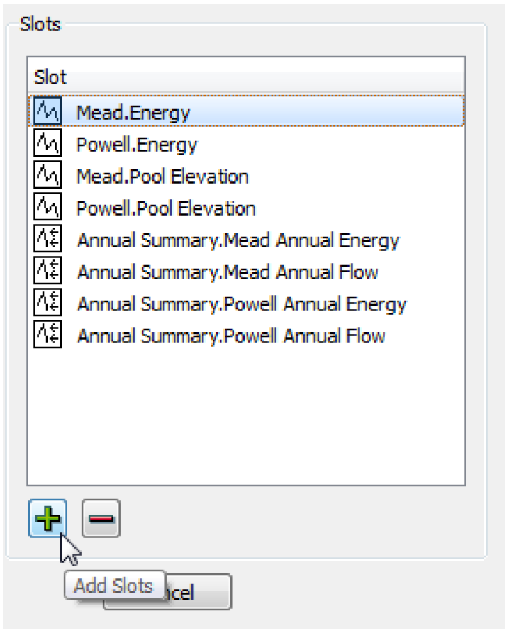
7. After configuring the netCDF output, select OK in the NetCDF File Configuration dialog, and select Apply or OK in the MRM Configuration dialog to apply the changes.
Revised: 01/11/2023