Solution Approaches

Solution Approaches : Multiple Run Management

Solution Approaches

Multiple Run Management

Multiple Run Management is a RiverWare utility for setting up and automatically running many runs. The runs are set up through the Multiple Run Manager, which then carries out all runs and outputs the results into an RiverWare Data Format (RDF) and/or Excel file or through an output DMI.

A multiple run is defined as a set of one or more model runs, for all runs:

• The model configuration (object network) remains constant.

• The timestep size is constant.

• The same set of slots is saved to the output.

Runs are conducted automatically; i.e., RiverWare controls and invokes each run without user interaction.

Running a Preconfigured MRM Model

This section describes how to run a preconfigured MRM model. It is assumed that the MRM configuration is already set up and you wish to run the multiple runs and view the multiple run output.

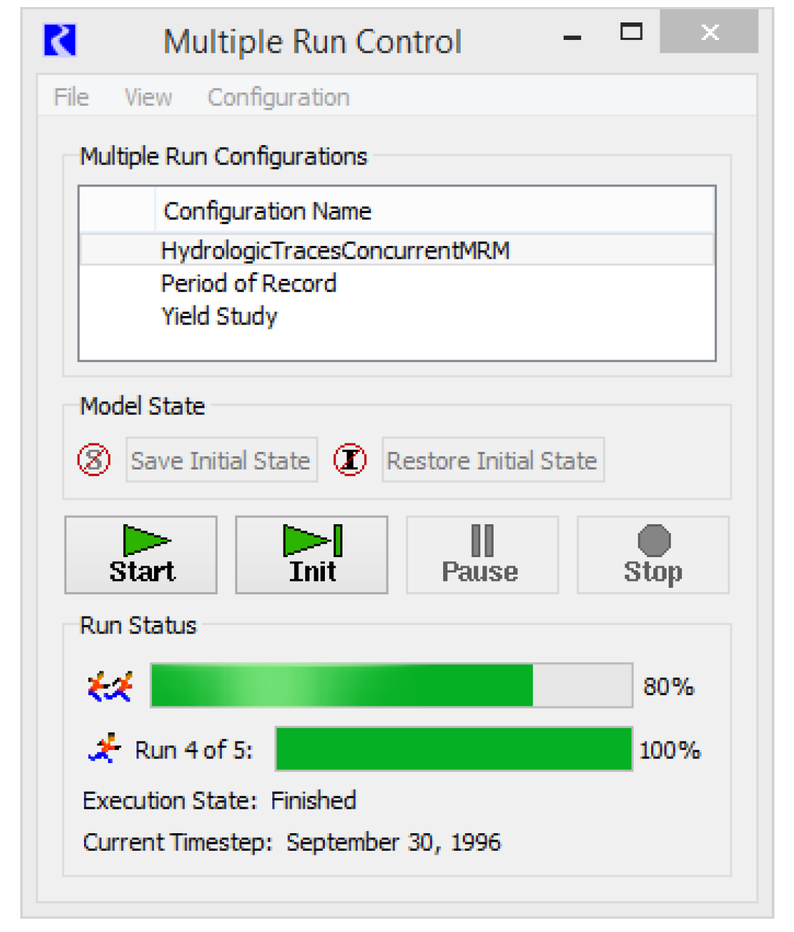
• Open the MRM Dialog by selecting Control, then MRM Control Panel from the main RiverWare menu bar or select MRM

on the toolbar.

• Highlight the desired configuration.

• Press the Start button.

• After the run has finished, determine where the output was placed by selecting Configuration, then Edit and selecting the Output tab in the ensuing Multiple Run Editor dialog.

– If there is a value in the Control File field this means that data was sent to the RDF file (or files) specified in the control file using the “file=” keyword. If there are no “file=” keywords specified in the control file, the data will go to the file specified in the Data File field. If Generate Excel files from RDF files is selected, an Excel spreadsheet was also created in the same folder and by the same name as the control file.

– If there is a value in the DMI field, this means that data was sent to a database using a DMI. Check the diagnostics output window for DMI diagnostics that show where output was sent. DMI slot diagnostics must be turned on during the run for this information to be printed.

See “Output” for details. See “RDF Viewer” for more information on quickly viewing the results of an MRM run using the RDF Viewer.

Managing MRM Configurations

This section describes how to manage MRM configurations using the Multiple Run Control dialog. The basics of creating, deleting, and opening a configuration for editing are described here.

• Open the MRM Dialog by selecting Control, then MRM Control Panel from the main RiverWare menu bar or select the MRM button on the toolbar.

Creating a New Configuration

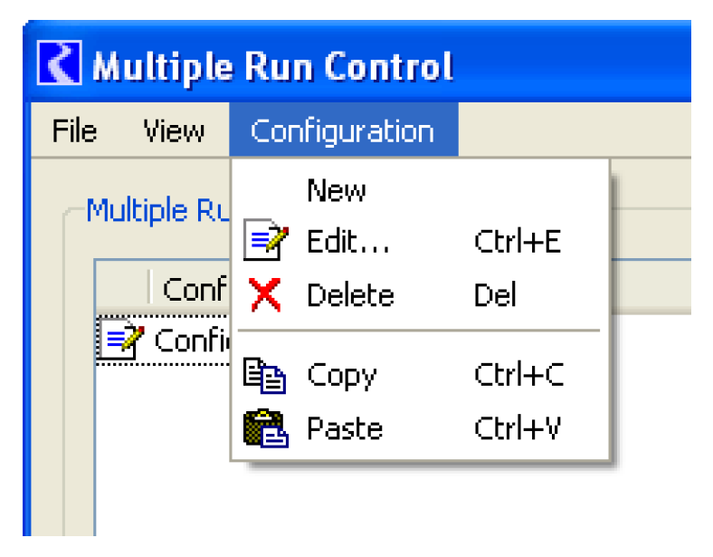
• Select Configuration, then New from the Multiple Run Control Dialog.

• Double-click the newly created configuration (or highlight it and select Configuration, then Edit or right-click the highlighted configuration to bring up a context menu and select Edit).

• In the MRM Configuration, make any necessary edits to the new configuration and select OK. See “Setting Up A Multiple Run Configuration”for details.

Editing an Existing Configuration

• Highlight the desired configuration in the Multiple Run Control dialog and select Configuration, then Edit or right-click the highlighted configuration to bring up a context menu and select Edit.

• Apply desired edits in the MRM Configuration dialog and select OK.

Deleting an Existing Configuration

• Highlight the configuration to be deleted and select Configuration, then Delete or right-click the highlighted configuration to bring up a context menu and select Delete.

• Apply the deletion by confirming the dialog

Copying an Existing Configuration

An easy way to create a new configuration similar to an existing one is by copying the existing configuration and making changes. Configurations can only be copy and pasted within one model (i.e., within one open session of RiverWare).

• Highlight the configuration to be copied and select Configuration, then Copy or right-click the highlighted configuration to bring up a context menu and select Copy.

• Select Configuration, then Paste to paste the copied configuration into the open Multiple Run Control dialog or right-mouse select the highlighted configuration to bring up a context menu and select Paste.

• Highlight the “Copy of” configuration and select Configuration, then Edit (or right-click the highlighted configuration to bring up a context menu and select Edit).

• Change the name, if desired, and make any other edits. Select OK in the Multiple Run Editor.

• Edit notations. Whenever a configuration is edited, the change is noted with an icon in the Multiple Run Control dialog until those changes have been either accepted or canceled.

Setting Up A Multiple Run Configuration

This section provides the steps to setting up a multiple run configuration. Setting up a multiple run configuration requires specifying several parameters in the MRM Configuration. The parameters and brief descriptions are provided below.

• Open the Multiple Run Control dialog by selecting Control, then MRM Control Panel from the main RiverWare menu bar or select the MRM button on the toolbar.

• Create a new configuration and edit an existing configuration, as appropriate. See “Creating a New Configuration” and “Editing an Existing Configuration” for details.

Name

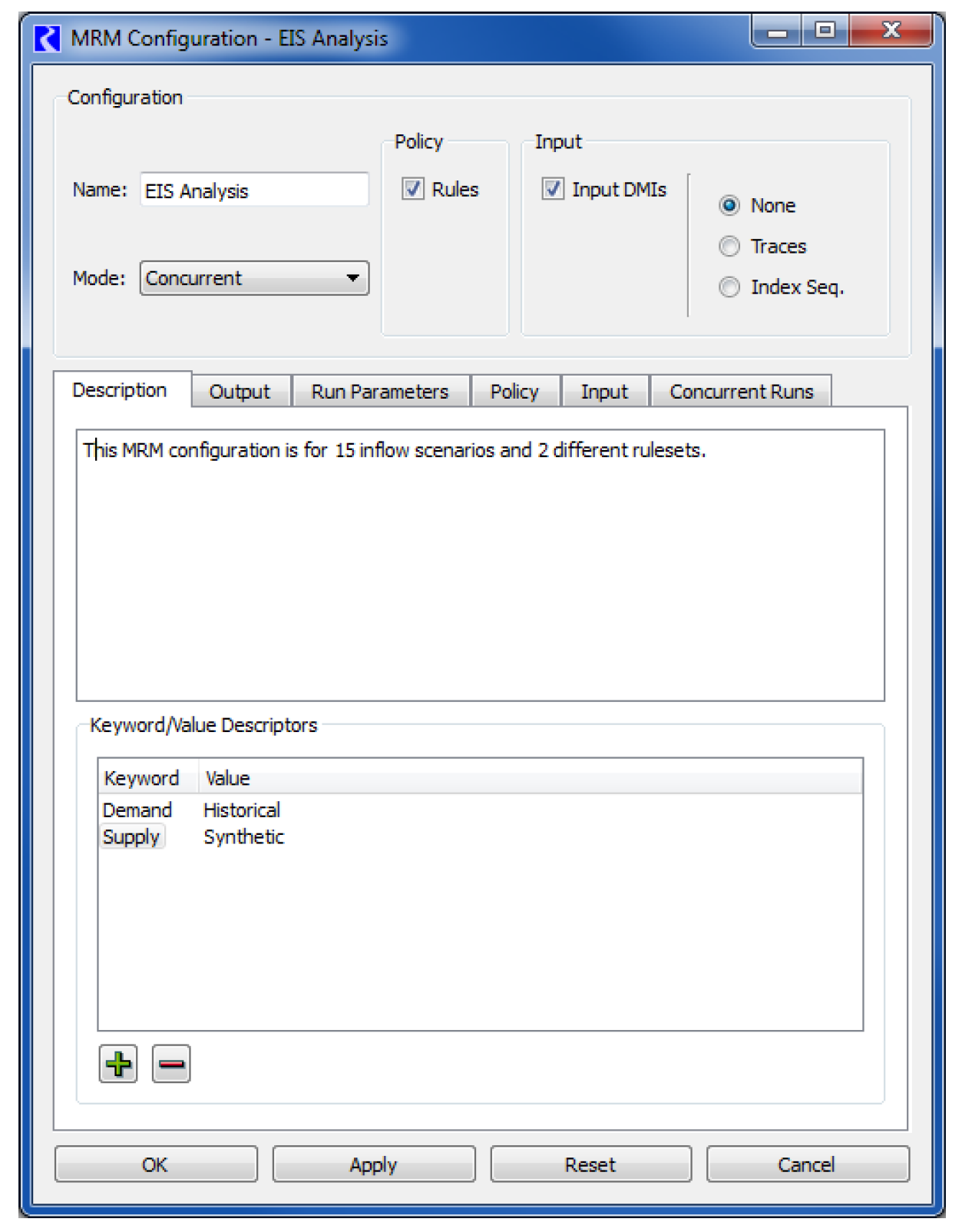
Provide a unique name for the configuration in the Name field.

Description

The configuration description in the upper panel may be multiple lines of text. This first non-blank line of the description appears in an MRM output RDF file. This text is optional, and will not affect the MRM execution if left blank.

Keyword/Value Descriptors are user-entered to describe the MRM configuration. For example, these could indicate something about the data being brought in by DMIs, something about the ruleset, or anything else the user would like to document. These descriptors can optionally be written into CSV or netCDF files output from the multiple run as described. See “CSV Files” and “NetCDF Files” for details.

Mode

Select the Mode of the configuration (Concurrent, Consecutive or Iterative) from the Mode menu. Selecting a mode will add the appropriate tabs to the dialog. Configuration of these tabs is described for each of the modes.

Concurrent Runs

Concurrent runs are multiple runs of which the time horizons are identical. The begin and end times, and timestep length, are the same for all runs. Concurrent runs are used to run the model multiple times with different inputs for each run. Inputs include rulesets (policy alternatives), input DMIs (i.e. series data like alternative hydrologies), and/or index sequential (data sampling technique).

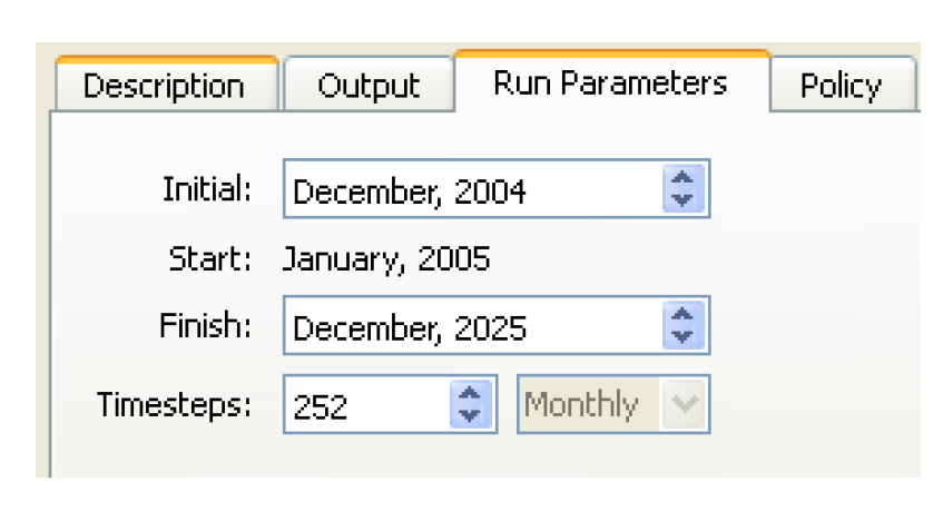
• For concurrent mode, the Run Parameters tab is shown. The Run Parameters tab describe the initial and end date of each concurrent run. The run parameters also show the timestep size but timestep size is dependent on the model and can only be changed in the single run control dialog.

Note: The Initial and Finish timestep for a concurrent run can be different than what is shown in the single Run Control.

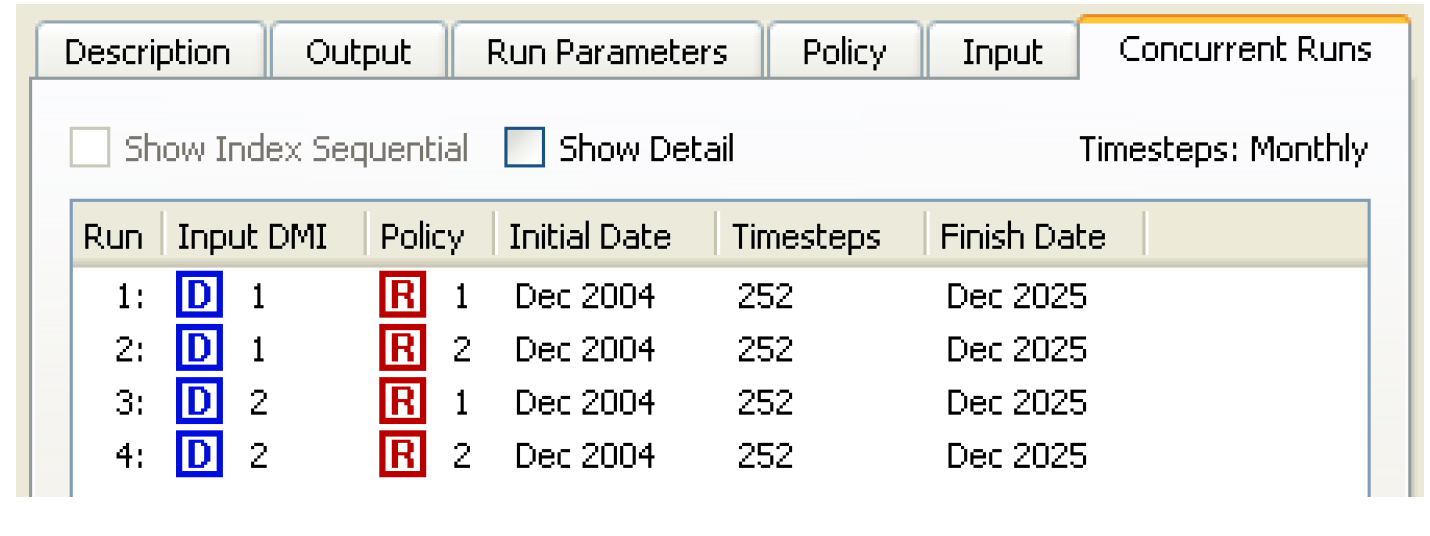
• The Concurrent Runs tab shows the number of runs that will be made.

– In most cases, the total number of runs should be the product of the number of rulesets, the number of input DMIs, and the number of index sequential runs:

#of MRM runs = #of Rulesets * #of Input DMIs * #of Index Seq Runs

– If the Pairs option for DMI/Index Sequential Mode has been selected on the Input tab, the total number of runs should equal the number of pairs of Input DMIs and Index Sequential runs. If the number of input DMIs does not match the number of Index Sequential runs, then the number of index sequential runs equals the total number of possible pairs, (i.e., the minimum of the number of input DMIs and the number of Index Sequential runs). (See the Index Sequential / DMI Mode section for more details.)

#of MRM runs = min(#of Input DMIs, #of Index Seq Runs)

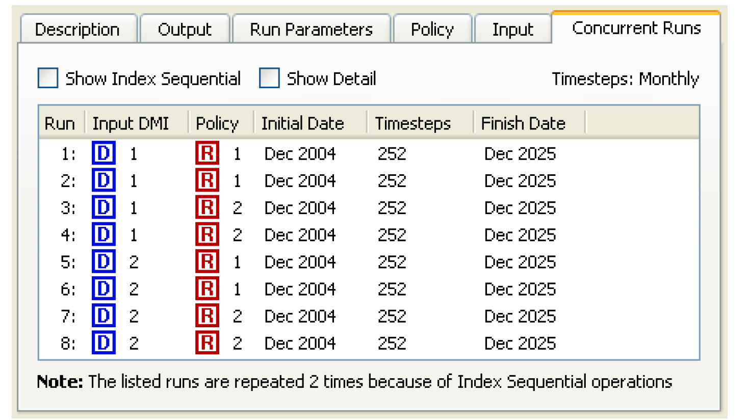
Figure 3.1 shows Concurrent Runs with 2 Input DMIs and 2 policy sets, no Index Sequential.

Figure 3.1

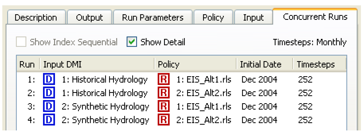
As shown in Figure 3.2, selecting the Show Details checkbox will show the names of the DMIs and policy sets.

Figure 3.2

Consecutive Runs

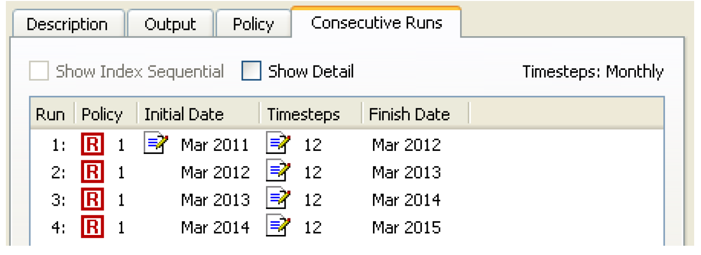
Consecutive runs are multiple runs where the time horizons are laid out consecutively. The end time of one run is the initial time of the next run. Timesteps do not vary among the different runs in a consecutive run.

• On the Consecutive Runs tab, the Edit button indicates which fields in this dialog are editable.

If necessary, change the Initial Date for the consecutive runs. Do this by selecting the existing initial date and toggling the up/down arrows in the ensuing date-time spinner.

• Change the number of timesteps for the first consecutive run by selecting the existing number of timesteps and toggling the up/down arrows of the ensuing integer spinner. The Finish Date automatically updates.

• Append a new row for each desired additional consecutive run by selecting the Plus button.

Or right-click below the existing consecutive run and selecting Append Row from the ensuing context menu. The Initial Date is automatically set to match the Finish Date of the previous consecutive run. In the Initial Date column, only the first consecutive run can be changed.

• Change the number of timesteps for each individual run, if necessary. The default is for newly appended runs to have the same number of timesteps as the previous run.

• To remove a run, select the Minus button. This will always remove the last run.

Iterative Runs

Iterative runs are multiple runs where MRM rules at the beginning and/or end of each run examine the state of the system and, if appropriate, set values for the subsequent simulation run. If no values are set or the maximum number of iterations occurs, then the simulation ends. As in concurrent runs, the time horizons, begin and end times and timestep length are all the same for all runs.

The iterative runs can use any of the controllers as specified in the single Run Control dialog: simulation (with or without accounting), rulebased (with or without accounting) or optimization. If the run is rulebased or optimization, the same RPL set or Goal set, respectively, is used in each iteration.

An iterative run executes as follows:

1. Initialize the iteration count.

2. Execute the Pre-MRM Run Rules, if specified.

Note: Pre-MRM Run Rules are similar to Initialization rules for each run; see “Initialization Rules Set” in RiverWare Policy Language (RPL).

3. Perform a single run.

4. Execute the Post-Run Rules, if specified.

5. If the Post-Run Rules return “no change”, that is they do not assign one or more new (different) values, the iteration is complete.

6. Otherwise, the iteration count is checked. If it equals the maximum number of iterations specified, then the iteration is complete also.

7. If the iteration is not complete, then increment the iteration count and return to Step 3..

When an MRM rule, either pre-run or post-run, sets a value on a slot, the value is given the i flag indicating that it is a “Iterative MRM” flag. Values with the iterative MRM flag are cleared at the beginning of an iterative MRM run but are not cleared between iterations of the MRM. This allows values set by the iterative MRM rules to persist between iterations but values are cleared at the beginning of the MRM run. In non-iterative MRM and single runs, values with an i flag are also cleared. You should be aware of this behavior if switching from iterative MRM to another mode.

Values set by the Iterative MRM “i” flag behave with output semantics. That is, they can be overwritten by any other value. In rulebased simulation, they are set when the controller is at priority zero, so values are given a priority of zero. Iterative MRM rules should only set values on data objects (typically integer indexed series slots as described at the end of this section), not simulation objects. Iterative MRM rules should be used to control the multiple runs; rulebased simulation rules within the run should be then used to set values on simulation slots that will actually be used in the run.

To configure an iterative run:

• Within the MRM Configuration dialog with the iterative mode, there is no Run Parameters tab. The iterative runs will begin at the start timestep of the model run. If users wish to change the model start timestep, this should be done in the single Run Control dialog.

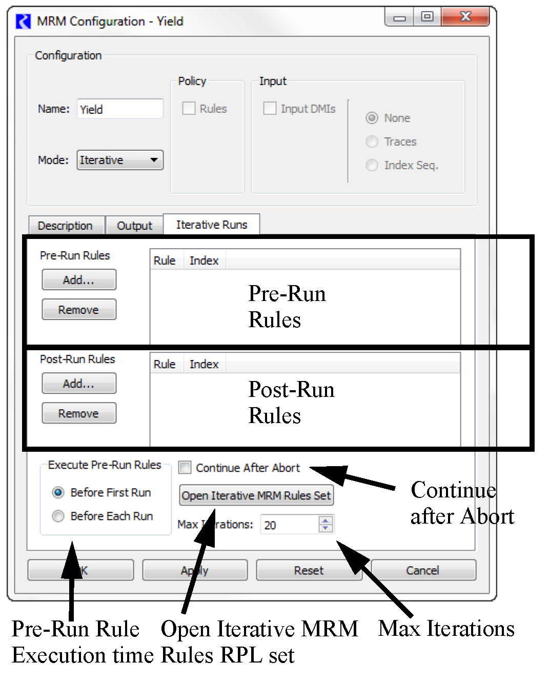
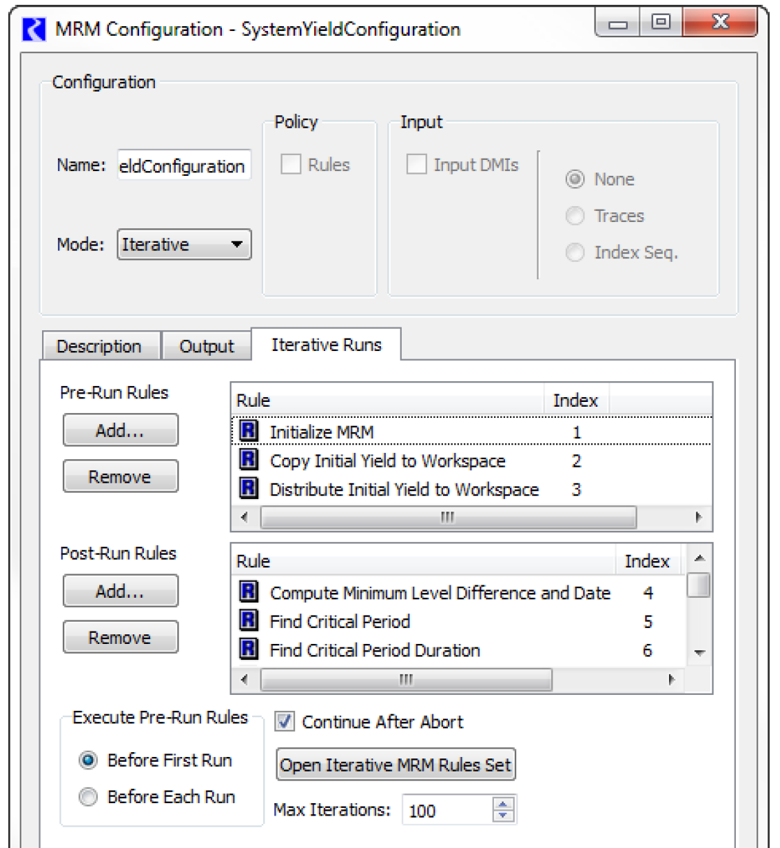
• On the Iterative Runs tab are the following significant areas: the Pre-MRM Run Rules, the Post-Run Rules, the Continue After Abort toggle, Pre-Run Rule Execution Time, the Open Iterative MRM Rules Set button, and the Max Iterations selector.

• Select Open Iterative MRM Rules Set button to open the Iterative MRM Rule set editor. This dialog operates very similarly to the standard RBS Ruleset Editor dialog. Create one (or more) Policy Group(s) and associated rules. The MRM Rules created are stored within the model file and may be available for use with any number of iterative MRM configurations. This set of rules can also be accessed from the workspace Policy, then Iterative MRM Rules Set.

• Once the MRM Rules have been built, return to the Iterative Runs tab of the MRM Configuration dialog. In this tab, the define which of the MRM rules should execute as part of the PreRun rules and which should execute after each iterative run, or both. These are defined in the appropriate areas using one of the following methods

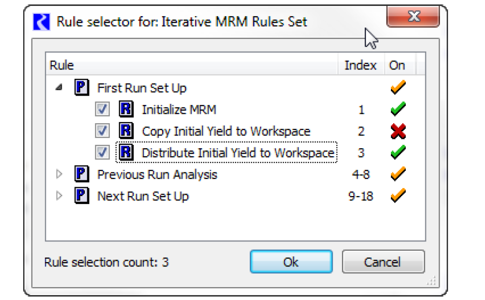
– Use the Add and Remove buttons. Select the Add button to bring up the Rule Selector as shown in the following figure. This dialog shows the rule groups in a tree view. Expand the tree-view to show individual rule names, their Index and their On status. Select the checkbox to check the desired rules. Select Ok to accept and return to the configuration dialog.

– Drag and drop rules from the MRM Ruleset to the Pre-Run Rules area or Post-Run Rules area.

Note: The order of addition into the display does not affect the rule ordering; the order is strictly consistent with priorities defined in the MRM Rules.

• To view a rule directly from the Iterative Runs tab, double-click the rule’s name to open the Rule Editor.

• Use the Execute Pre-Run Rules buttons to specify when Pre-Run Rules are executed:

– Before First Run. This is the default. Choose this option to execute the Pre-Run Rules before the first single run only, but not before subsequent runs.

– Before Each Run. Choose this option to execute the Pre-Run Rules before each single run.

• Consider activating the Continue After Abort option. If you want the Post-Run Rules to execute and possibly the next iteration to begin after an iteration is prematurely aborted (for any reason), select the checkbox.

• Select the Max Iterations selector and adjust it using the up and down arrows or by typing a value in the field to define the maximum number of iterations to run. Figure 3.3 shows a fully configured Iterative Runs tab.

Figure 3.3

Note: The Post-Run Rules must make a significant change in values (for example, through a rule assignment or import of data through an input DMI) at the end of each run for the controller to make the next iteration. If the Post-Run Rules do not set any values, (possibly due to convergence) the controller will assume that the goal of the iterations has been achieved and stop.

Note: The MRM rules execute differently from the basic ruleset. When the MRM rules execute, each fires once and only once according to the execution order specified. There is no dependency functionality. In fact, they will all fire even if one of them aborts.

Integer indexed Series Slots work very well with Iterative MRM. Using these slots, you can store inputs, outputs, or intermediate results based on the index of the run. For example, after each iterative run, you could store the total volume of water released in an integer index slot in the row corresponding to the run index. At the end of the entire run, all of these volumes are stored and can be reviewed. The GetRunIndex predefined function can be used to get the index of the next iterative run. See “Integer-indexed Series and Agg Series Slots” in User Interface and “GetRunIndex” in RiverWare Policy Language (RPL) for details.

Policy

For concurrent and consecutive mode, rulesets can be specified for the runs. The policy setup of the configuration (None or Rules) must be selected from the Policy section of the MRM Configuration. Selecting Rules will enable the Rulebased Simulation controller when the multiple run is started. Rulebased multiple runs are runs in which there are one or more rulesets. You specify the ruleset to use for each run. Variations in rules can be a function of differences in content, priorities, or both.

• Select Rules under in the Policy section of the MRM Configuration and select the Policy tab.

• Append a new row for each additional ruleset by selecting the Plus button

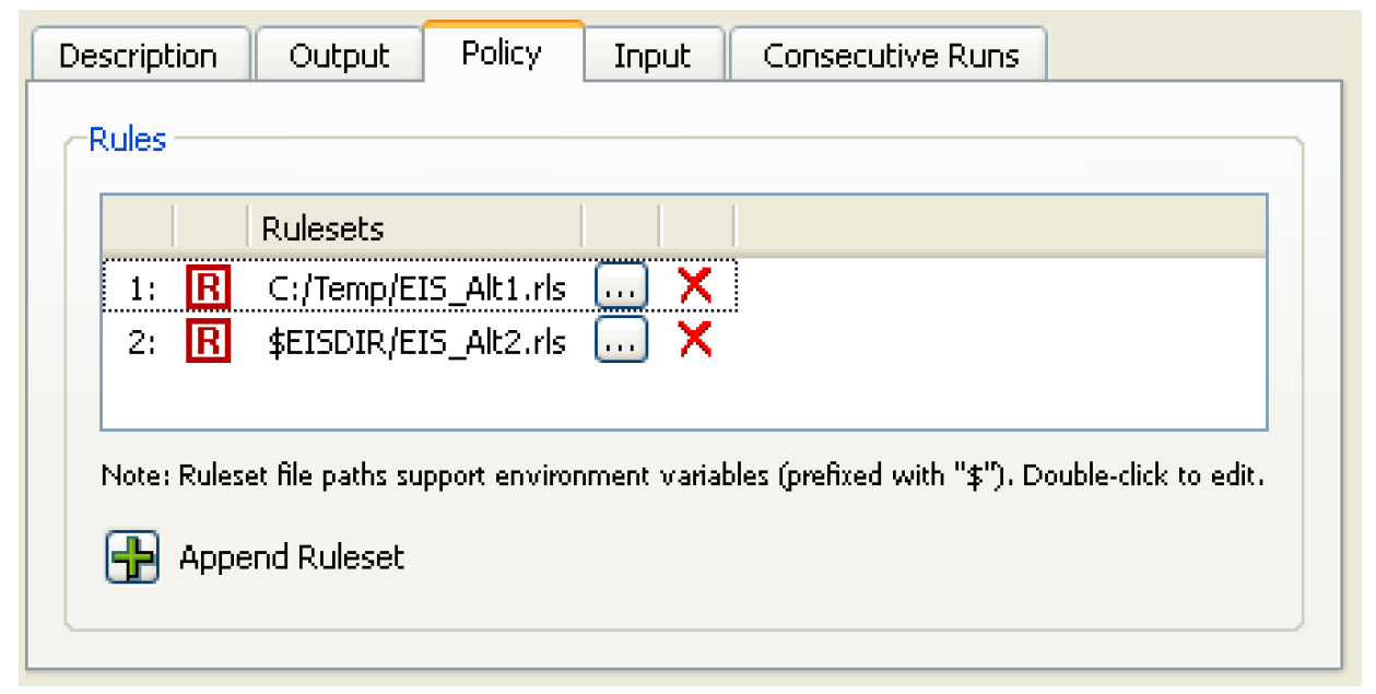
at the bottom.

• Select the ruleset by selecting the File Chooser button

or double-click and type in the path name of the ruleset directly. This allows you to use environment variables in the path. Environment variables are prefixed with the “$”.

• If necessary, remove a ruleset by selecting the Delete button

. There is no confirmation, but you can restore ruleset rows using the Reset button.

In Figure 3.4, the first ruleset was specified by browsing to the C: drive, the second ruleset was specified by typing the path in directly and using the environment variable EISDIR

Figure 3.4

Note: The Policy tab is not applicable to Iterative MRM runs, but an iterative run can be a rulebased run where one ruleset is used for all iterations. It must be explicitly opened and loaded before the iterative run is started.

Note: Multiple rulesets in a single MRM configuration are not supported if using Distributed Multiple Runs; see “Distributed Concurrent Runs” for details.

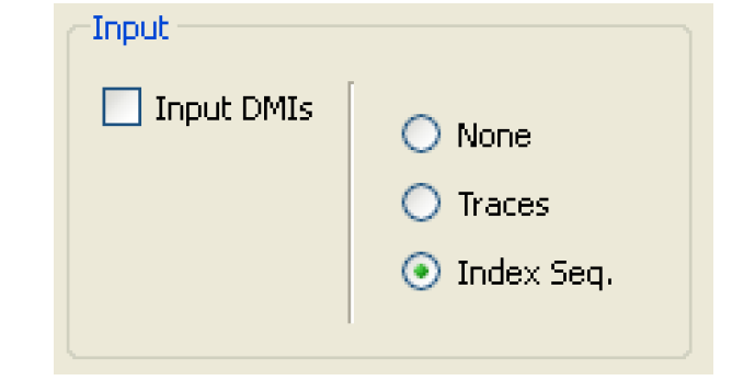
Input

The inputs to the multiple runs are specified by selecting options in the top of the dialog and then specifying configuration details in the appropriate tabs.

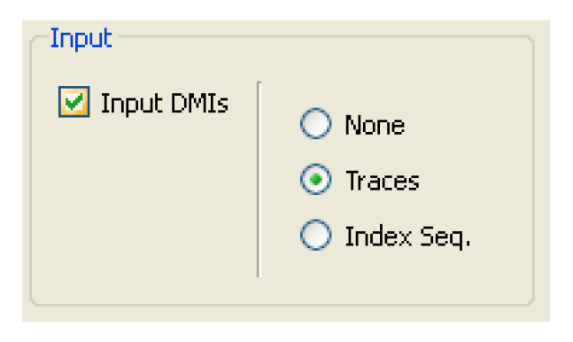
• If the Multiple Runs use an Input DMI, select the Input DMIs checkbox in the Input section.

• Optionally specify one Initialization DMI; see “Initialization DMI”.

• Specify whether to use Traces, Index Seq., or None. See “Index-sequential Runs” for details on Index Sequential. See “Input DMI Runs” for details on traces.

Note: The Input section and tab are not applicable or available to Iterative runs.

Initialization DMI

You can optionally specify a single DMI or group that is invoked at the beginning of the multiple run. Select the Initialization DMI toggle to show the entry field. Type in the name of an existing DMI or use the

button to select an the DMI or group.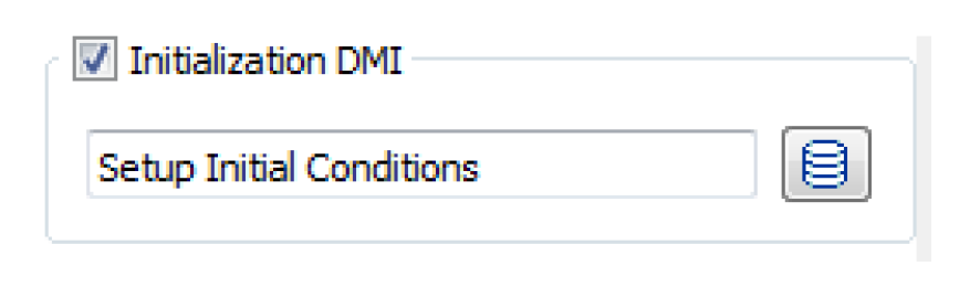

Input DMI Runs

Input DMI runs vary the input data for a specified set of slots. For instance, ten runs might represent ten alternative release schedules for a reservoir. You specify the number of runs and a DMI for each run. The DMI loads the data into the model for each run. The DMIs must be previously defined in the RiverWare DMI interface.

• When the Input DMIs is selected on the MRM Configuration, on the Input tab, the Input DMIs section becomes active.

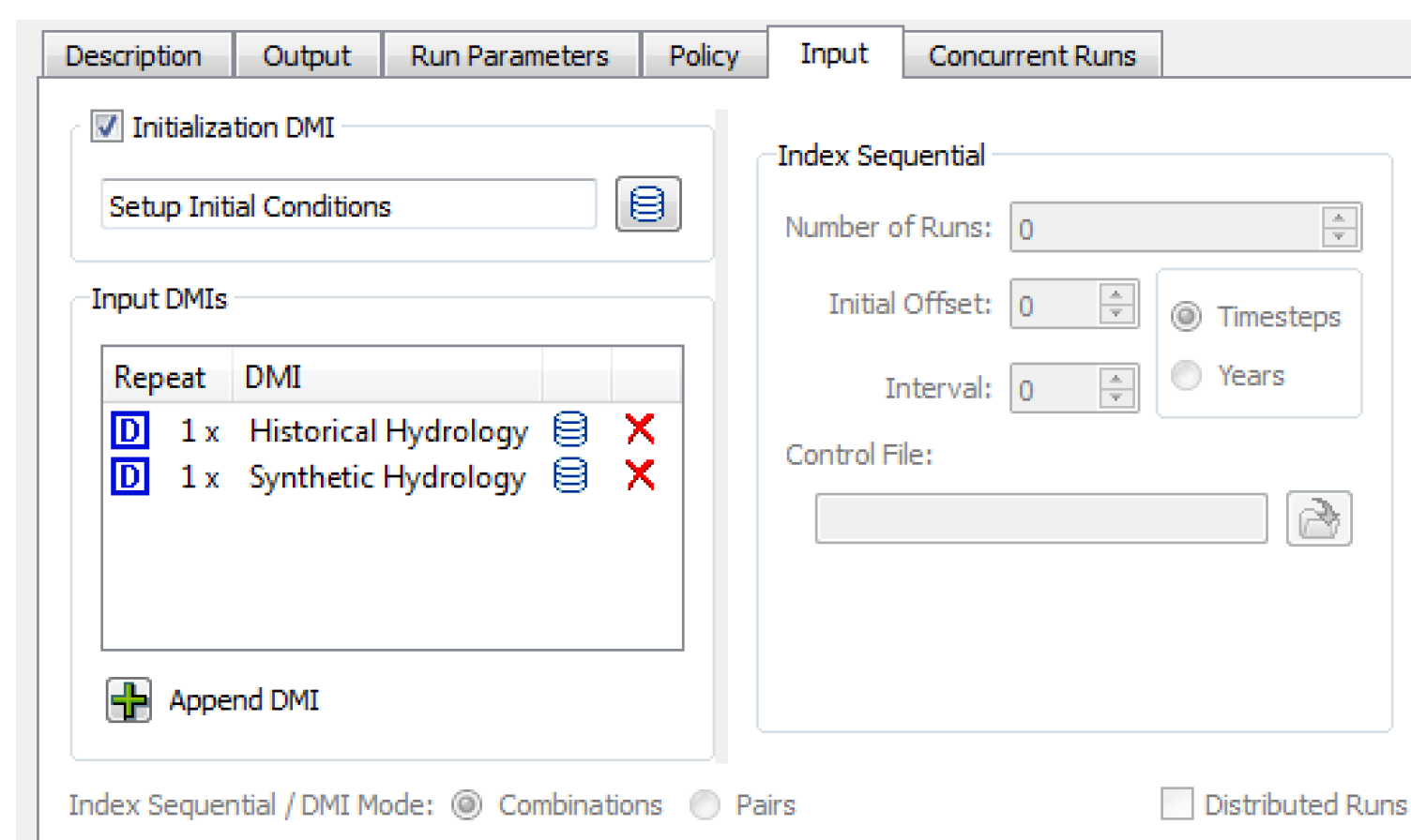
• Append a new DMI by selecting the Plus button

at the bottom

• Select the input DMI by selecting the DMI icon

and then choosing the previously configured DMI from the list.

• If the DMI will be called more than one time, change the number in the Repeat column by double-clicking the cell and using the up/down arrows. DMIs might need to be called more than once in a MRM run, for example, with runs that execute multiple traces using the same DMI. In this situation, the DMI needs to be configured to make use of the trace number.

– For a Control File-Executable DMI, the executable should reference the last command line parameter passed from RiverWare:

-STrace=traceNumber

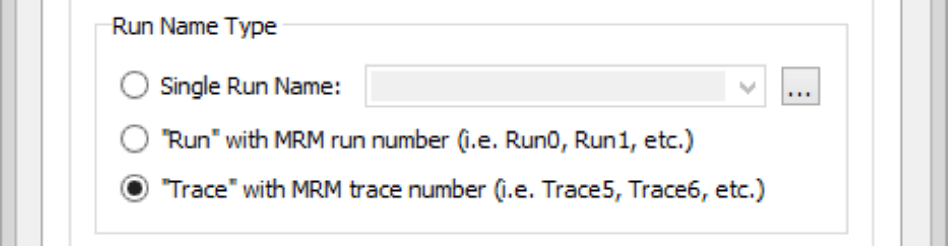
– For an Excel DMI, the Excel Dataset Run Name Type setting should use either the Run or Trace option; see “Run Name Type” in Data Management Interface (DMI).

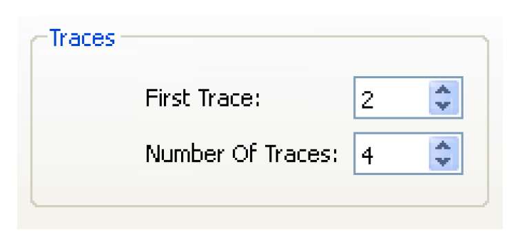
• If you are using Input DMIs but not using Index Sequential, you can choose the Traces option from the Input section on the MRM Configuration. This allows you to run only a portion of the runs specified by the Input DMIs. When Traces are specified, the Input tab shows the Traces area. In this area, you can specify

– First Trace

– Number of Traces

– To not run a subset of the runs, select None.

• If you wish to use Ensembles with HDB datasets, select the Input Ensembles checkbox. See “Ensembles” for details.

Index-sequential Runs

Index Sequential runs use an input time series which is systematically shifted between runs. You specify the number of runs, the interval (number of timesteps) by which the input data is shifted from one run to the next, and an initial offset (number of timesteps) by which data is shifted for the first run. The slots with input data to be shifted are identified by in a DMI control file. This type of run is typically used to perturb (shift) historical hydrologic data in order to be able to conduct statistical analysis of the results.

Note: Index Sequential is not applicable to Iterative or Consecutive runs.

Index Sequential specifies that, given a run start time, run timestep, run duration, number of runs, and time offset, input time series, a run can be systematically perturbed between runs. For example, if an Index Sequential run is defined as the following:

• input time-series:

• original value vector: 1, 2, 3, 4, 5, 6, 7, 8, 9

• original time vector: Jan, Feb, Mar, Apr, May, Jun, Jul, Aug, Sep

• offset: 4 timesteps

• interval: 1 timestep

• number of runs = 3

then, the following sequence of runs occurs:

• Run 1: Jan = 5, Feb = 6, Mar = 7, Apr = 8, May = 9, Jun = 1, Jul = 2, Aug = 3, Sep = 4

• Run 2: Jan = 6, Feb = 7, Mar = 8, Apr = 9, May = 1, Jun = 2, Jul = 3, Aug = 4, Sep = 5

• Run 3: Jan = 7, Feb = 8, Mar = 9, Apr = 1, May = 2, Jun = 3, Jul = 4, Aug = 5, Sep = 6

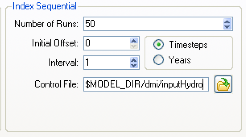
To setup an Index-sequential run:

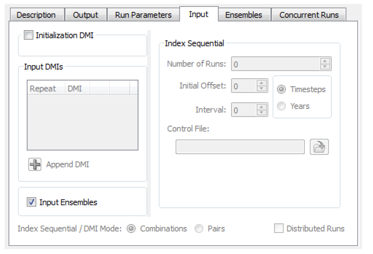
• Select Index Sequential in the Input section of the MRM Configuration and select the Input tab.

• Specify the Number of Runs by typing in the value or by toggling the up/down arrows.

• Specify the Initial Offset by typing in the value or by toggling the up/down arrows.

• Specify the Interval by which the data is shifted from one run to the next by typing in the value or by toggling the up/down arrows in the Interval field.

• Specify the units for the Initial Offset and Interval as Timesteps or Years.

• Specify the Control File by typing in the path directly or by using the file chooser to select it. Typing in the path and name directly allows for the use of environment variables. Take care to spell the entire path correctly. The control file specifies the slots that will be rotated for each run. It uses the same format specified, but no file name or keyword value pairs are necessary. Typically, it is just the object and the slots that are specified. See “Control File” in Data Management Interface (DMI) for details.

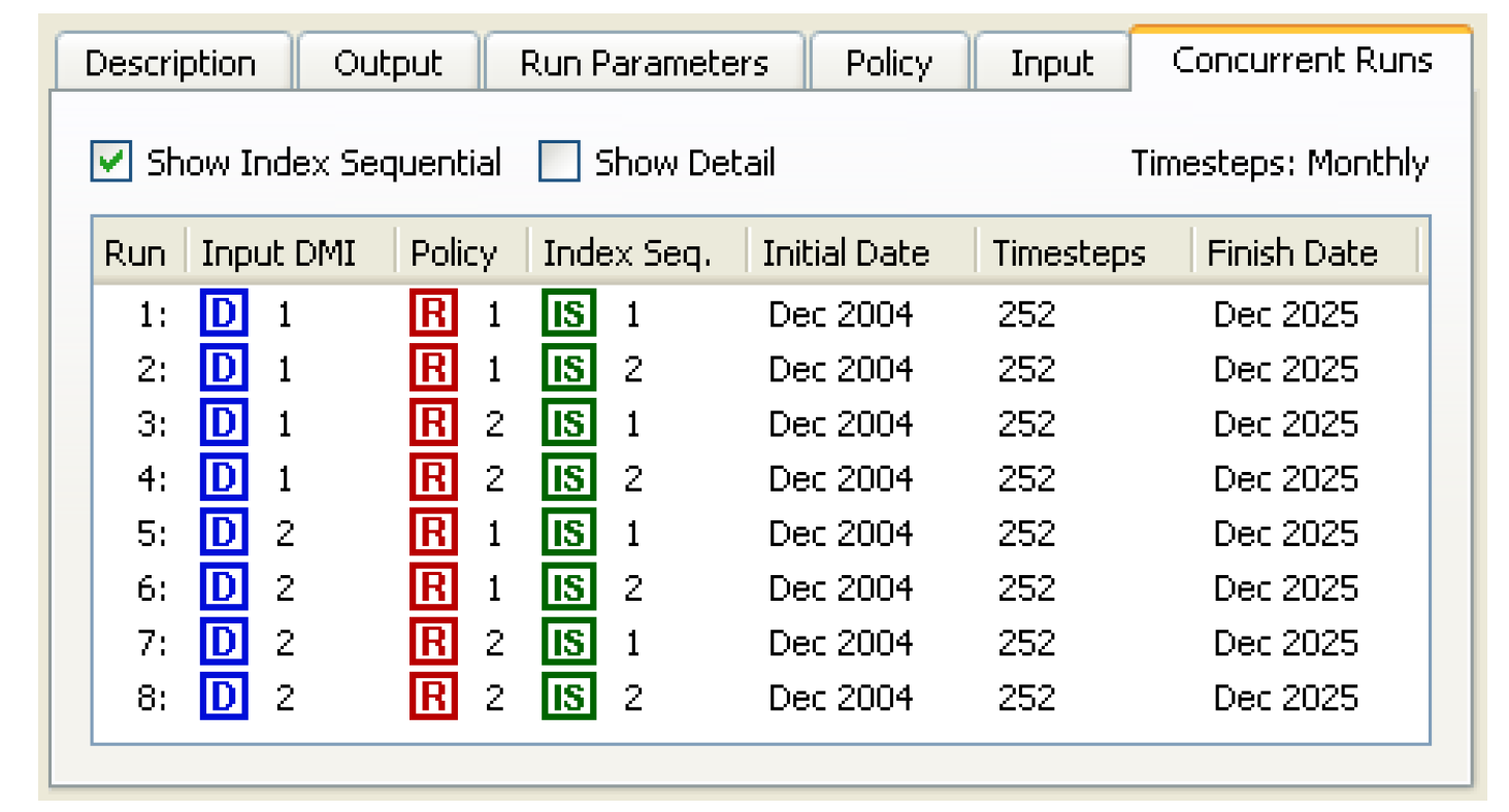
• On the Concurrent Runs tab, the combinations of policy sets and Input DMIs are set up for the index sequential run.

• Select the Show Index Sequential checkbox at the top of the Concurrent Runs tab to view each index sequential run listed individually.

Combined Runs

By default, the runs that are made in concurrent MRM are a multiplicative combination of inputs. This set is called Combined Runs. Combined runs are defined as the Cartesian product of all the involved base-type runs. For example, a combined run consisting of two rulesets and four Input DMIs, results in 2 * 4 = 8 model runs.

The order in which individual runs within a combined multiple run are executed is determined by the precedence level of each mode. Order of precedence (from highest (1) to lowest (3)) is as follows:

1. Input DMI runs,

2. Rulebased runs, and

3. Index-Sequential

Elements of lower precedence iterate before elements of higher precedence. For example, in case of a combined run containing two Input DMI runs and two Rulebased runs, the following sequence of four runs is made:

1. Input DMI 1 & Ruleset 1.

2. Input DMI 1 & Ruleset 2.

3. Input DMI 2 & Ruleset 1.

4. Input DMI 2 & Ruleset 2.

Thus, the default combinations mode results in the total number of runs equal to the product of the number of policy sets, the number of input DMIs, and the number of index sequential runs:

#of MRM runs = #of Policy Sets * #of Input DMIs * #of Index Seq Runs

In very specific circumstances, it is possible to alter the mode of how many MRM runs result from the combination of input DMIs, policy sets, and Index Sequential runs. If Index Sequential has been selected and there are as many (or more) Input DMIs as Index Sequential runs and there are zero or one rulesets selected, then it is possible to choose either Combinations or Pairs in the Index Sequential / DMI Mode selection.

The Pairs mode results in the total number of runs equaling the number of pairs of Input DMIs and Index Sequential runs. If the number of input DMIs does not match the number of Index Sequential runs, then the number of index sequential runs equals the total number of possible pairs, (i.e., the minimum of the number of input DMIs and the number of Index Sequential runs). The Pairs mode is necessary to run the CRSS Lite model.

# of MRM runs = min(# of Input DMIs, # of Index Seq Runs)

When the pairs mode is specified, the runs can be distributed to multiple processors. See “Distributed Concurrent Runs” for details.

Ensembles

An ensemble contains a set of traces where each trace represents the data for one run of the multiple run. An ensemble of trace data can function as input to the runs of a multiple run, or can represent output from a multiple run. An ensemble can have metadata that describes the overall ensemble and metadata that describes each of the individual traces.

Note: Currently only HDB datasets in Database DMIs can be configured to function as ensembles.

Ensemble Configuration

To utilize ensembles, on the Input tab of the MRM configuration, select the Input Ensemble checkbox. This will disable Input DMIs, Traces, and Index Sequential functionality as the ensembles will determine the number of runs in the multiple run.

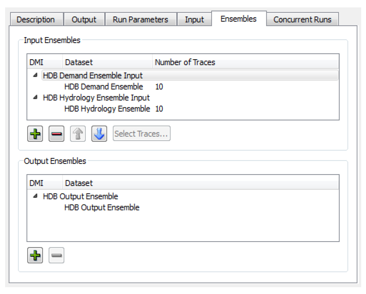
When you select the Input Ensembles toggle, an Ensemble tab is added to the dialog where input and output ensembles are specified.

Select the Plus in the Input Ensembles frame to open a list of input DMIs defined in the model. You can select one to add as an ensemble. Only valid input DMIs with datasets configured with ensembles can be added.

Note: Currently only HDB datasets in Database DMIs can be configured to function as ensembles. See “HDB Table Type—Ensembles” in Data Management Interface (DMI) for details.

Input DMIs will be executed in the order shown. This allows you to configure how data is loaded if the same slots are used in multiple input DMIs (the last one in wins). Use the up and down arrow buttons to reorder the selected DMI.

When a DMI is added as an input ensemble, it defaults to using all of the traces defined in the ensemble. The number of traces is shown for the DMI, or for its datasets in the case of database DMIs, as a column in the dialog. When an item having traces is selected in the list, the Select Traces button is enabled. Select this button to open a dialog showing all of the traces for the ensemble. Choose a subset of traces as desired.

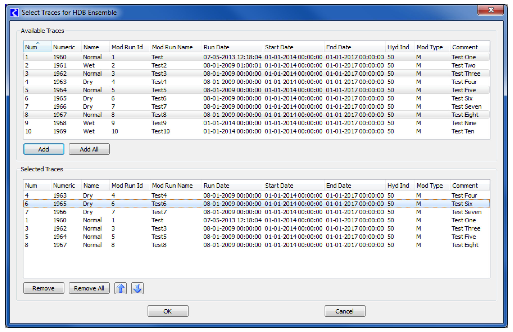
All available traces are presented in the upper list. When added using the Add or Add All buttons, they are copied to the lower list showing the selected traces. Traces can be removed from the selected list with the Remove or Remove All buttons. The selected traces can be ordered using the up and down arrow buttons. With these controls, a subset of traces in the ensemble can be chosen and used in any order as input to the multiple run. When applied with the OK button, the number of selected traces will now appear in the Number of Traces column in the Input Ensembles frame of the Ensemble tab.

The number of traces for input ensembles must match across all of the input ensembles because the number of traces input to the multiple run will determine the number of runs. If an MRM configuration with differing numbers of input ensemble traces is applied or a run is started, an error message is generated.

HDB ensemble datasets have an option to defer picking an ensemble for the dataset until the MRM run is started. See “HDB Table Type—Ensembles” in Data Management Interface (DMI) for details. In this case, the Number of Traces column will show a zero, and using the Select Traces button will return a message that the ensemble will not be selected until MRM start. Where datasets of this type are used in input ensembles, the number of runs in the multiple run cannot be determined until the MRM run is started, so the Concurrent Runs tab of the MRM configuration dialog will be empty. Uniformity of number of traces across input ensembles is checked after ensembles are selected at the start of the MRM run.

DMIs to use as output ensembles are added and removed with the plus and minus buttons in the Output Ensembles frame of the Ensembles tab. Unlike input ensembles, the order of output ensembles does not matter, so there are no ordering controls in this frame. All existing data and metadata in output ensembles for a multiple run are cleared at the beginning of the multiple run. At the end of each run in the multiple run, the data specified in output ensemble DMIs are written to the trace of the output ensemble that corresponds to that run. An output ensemble must have at least as many traces as the number of runs in the multiple run so that all of the run data can be written. If an HDB dataset configured to select the ensemble at MRM start is used in an output ensemble, its number of traces is checked after the ensemble is selected.

Ensemble Metadata

An ensemble can have metadata that describes the ensemble as well as metadata that describes each trace in the ensemble. Metadata is represented in RiverWare as Keyword/value pairs, such as “comment”/”Climate Change Hydrology”. An important functionality of ensembles with MRM is that the ensemble and trace metadata from input ensembles are combined and copied over to output ensembles.

For ensemble metadata, values for the “domain”, or “comment” keywords from input ensembles are concatenated with semicolons and written as values for these keywords to output ensembles. For example, if there were two input ensembles, one with a comment “Historic Hydrology” and the other with a comment “High Projected Demand”, an output ensemble would be given the comment keyword value of “Historic Hydrology;High Projected Demand”. Values for other ensemble metadata keywords are not concatenated. If values for these other keywords differ among input ensembles, the keyword value from the first ensemble is copied to the output ensemble and a warning issued that values for this keyword differ among the input ensembles.

For trace metadata, values for the “name” keyword for multiple input ensemble traces will be concatenated with semicolons and written as the value for the “name” keyword to an output trace. Values for other trace metadata keywords are not concatenated. If values for these other keywords differ among multiple input ensemble traces, the keyword value from the trace of the first ensemble will be copied to an output ensemble trace and a warning issued that values for this keyword differ among the input ensemble traces.

See “HDB Table Type—Ensembles” in Data Management Interface (DMI) for details on HDB ensembles and metadata.

Output

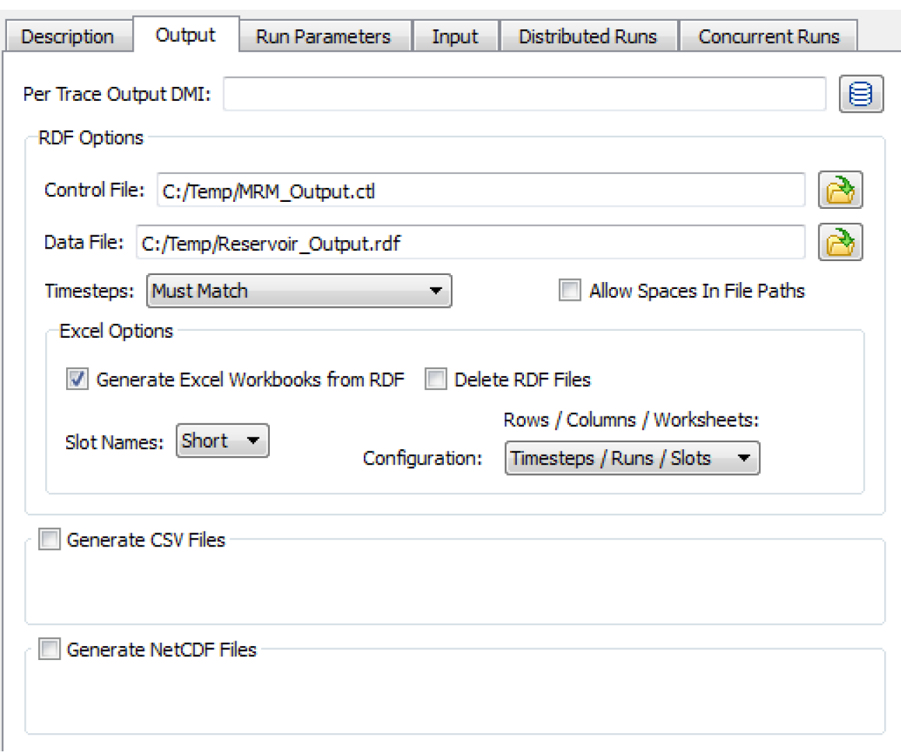
During a multiple run, output can go to an output DMI and/or one or more RiverWare Data Format (RDF) text files. Options are also available to send output to CSV files or NetCDF files. Select the Output tab of the Multiple Run Editor. The following are configuration options:

DMI

The optional Per Trace Output DMI field allows selecting or entering an output DMI or a group of output DMIs that will be run after each single run of the multiple run. HDB ensemble datasets cannot be used in these DMIs, but rather must be used in the MRM ensemble configuration; see “Ensemble Configuration” for details.

The DMIs must be previously configured in the DMI Manager in RiverWare. The executable that is configured for the DMI can reference the trace number of the run that is outputting by referencing the last command line parameter passed from RiverWare:

-STrace=traceNumber

Note: Using a Per Trace Excel Output DMI in combination with Distributed MRM is not recommended. In that case, multiple RiverWare processes can end up trying to write to the same Excel file simultaneously, which may cause a conflict. See “Distributed Concurrent Runs” for details.

RDF

Configurations for RDF output from MRM include the following:

Control File

Type or use the File Chooser button to select a complete file path into the required control file field. The control file is used to specify which slots are output after each MRM run. The control file may contain “file =” specifiers for any line entries in the file. This causes data associated with those lines to go to the specified RDF output file. In the example control file below, if “fileName” is the same for each slot, then the output will go to a single RDF file; varying fileNames will send the output to multiple RDF files.

MountainStorage.Inflow: file=fileName

MountainStorage.Outflow: file=fileName

MountainStorage.Storage: file=fileName file=fileName2

You can optionally specify multiple files for a single slot as in the third line above. Also, slots with a timestep different than the model’s timestep can be output using the same syntax.

In the control file, there are four ways to specify where the data files are created:

• Hard code the path: file=C:/DMI/Data/ResA.Inflow

• Use an environment variable: file=$(DMI_DATA)/ResA.Inflow

• Use '~': file=~/ResA.Inflow where '~' is replaced with $RIVERWARE_DMI_DIR/<DMI name>

• If the filename is not specified, the output file will be created in the directory in which RiverWare resides.

The second option is recommended as it is more transparent than '~” but still allows the model to be moved from machine to machine by setting the environment variable to the appropriate value on each machine.

Tip: See “RDF Viewer” for more information on quickly viewing the results of an MRM run using the RDF Viewer.

Timesteps

Specify whether RDF output files may contains slots whose timesteps differ. There are three choices:

• Must Match. All slots written to an RDF file must have the same timestep. Slots whose timesteps differ from the file’s timestep are skipped. (The file’s timestep is determined by the first slot MRM associates with the file.) You are warned about slots being skipped, and asked whether to continue the MRM run.

• Use Smallest. Slots written to an RDF file may have different timesteps, with the output written using the smallest timestep.For example, if slots with 1 Month and 1 Year timesteps are written to an RDF file, monthly values will be written and the 1 Year slots will write 11 NaN followed by a value.

• Use Largest. Slots written to an RDF file may have different timesteps, with the output written using the largest timestep. For example, if slots with 1 Month and 1 Year timesteps are written to an RDF file, yearly values will be written and the 1 Month slots will write December values.

Data File

Optionally type or use the File Chooser button to select a complete file path into the Data File field. This file is used as the RDF output file for any lines in the control file that do not have an explicit file specifier. If the data file field is used and there are no “file=” specifiers in the control file, then all output will go to this single data file.

Excel Options

Select Generate Excel Workbooks from RDF to create Excel files from all of the RDF output files after all runs have completed.

Select Delete RDF Files to delete all RDF files after the Excel files are created. (The separate RdfToExcelExecutable program contains the same functionality for creating Excel files from RDF files and can be used outside of RiverWare to process RDF files from an MRM run.)

Select a Configuration from the menu to control how timestep, slot, and run data from RiverWare are mapped onto the Excel dimensions of rows, columns, and worksheets.

Select an option from the Slot Names menu to specify how slot names are written into the Excel workbook. Options are as

• Index: (Slot0, Slot1, etc.)

• Short: Automatically shortened names (lower case vowels removed)

• Full: Full slot names (limited to 31 characters for worksheet names, which is the limit for Excel)

CSV Files

CSV files can be generated from the MRM run outputs. The CSV files are formatted for direct use within Tableau data visualization software. The configuration allows for the selection of various pieces of information to be used as dimensions in Tableau. The CSV output is essentially a table with the columns delimited by commas.

1. Near the bottom of the Output tab in the MRM configuration dialog, select the checkbox for Generate CSV Files.

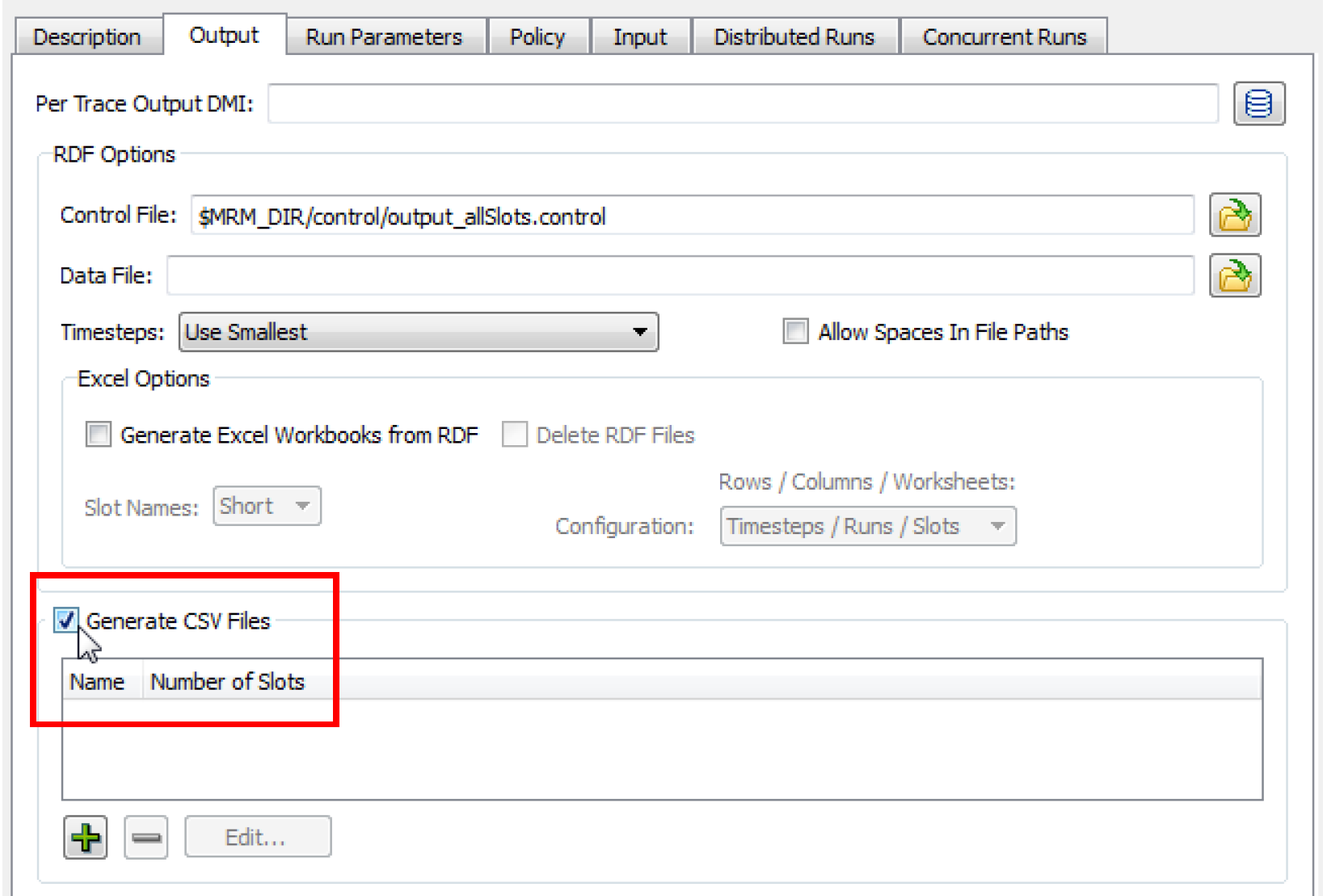
2. Select the Plus sign to add a new CSV output file. Then select Edit to configure its contents. This will open the CSV File Configuration dialog.

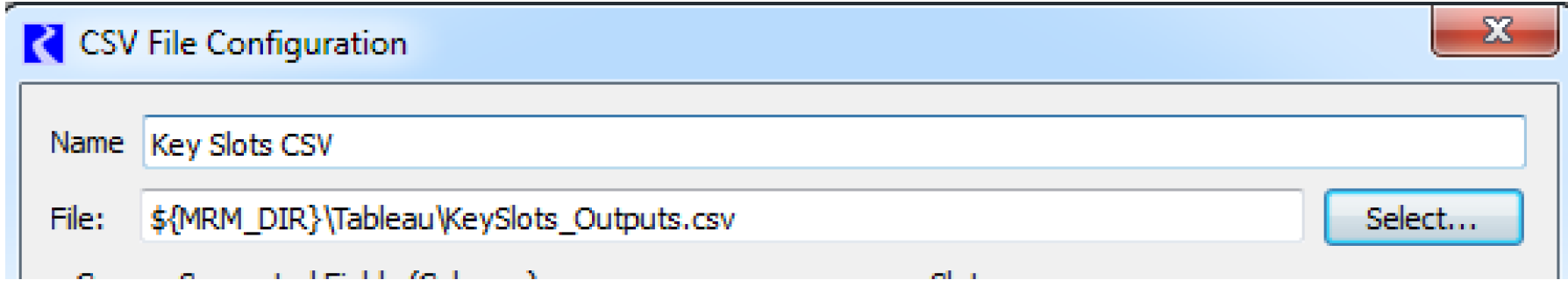
3. The CSV can then be given a name to display in the list in the MRM configuration.

4. In the File field, either select a CSV file to which the new outputs should be written by selecting the Select button, or type in a complete file path. Environment variables can be used in the file path preceded by a “$”.

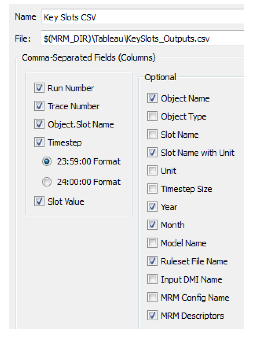
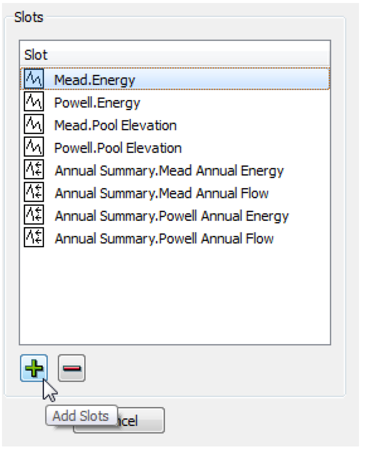
5. Next, select which pieces of additional information should be included as columns in the output table by selecting or clearing the checkbox by each optional element. Figure 3.5 shows the list of available elements. The CSV output file will contain a column for each item selected. The text shown in the CSV File Configuration dialog will be used as the column header. The Slot Value column is the only column that will contain true “output” data from the MRM run. The Slot Value will be considered a “measure” within Tableau. The remaining columns contain information associated with each Slot Value and will be considered dimensions within Tableau.

Figure 3.5

Note: In the context of Distributed Multiple Runs the Run Number corresponds to the run number on the individual processor. Thus if there are eight runs distributed to four processors (two each), all rows in the resulting CSV file will show a Run Number of either 1 or 2.

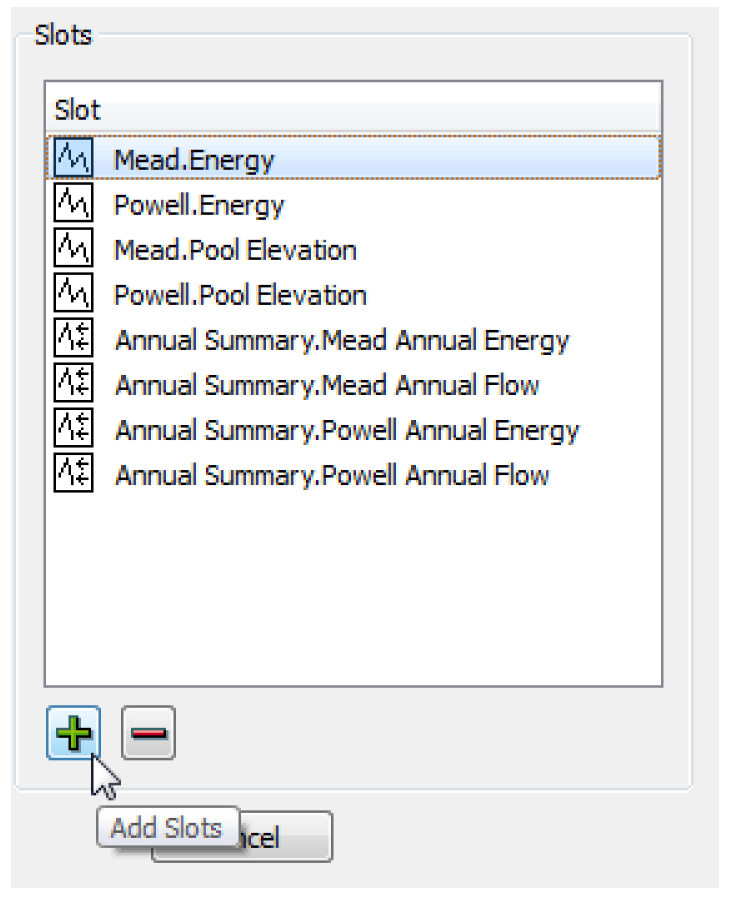
6. Then add slots to the CSV output by selecting Plus sign below the Slots panel. This will open a slot selector dialog, which can be used to add the desired slots. A slot can be removed from the selection by selecting it in the list to highlight it, then selecting the Minus sign.

7. After configuring the CSV output, select OK in the CSV File Configuration dialog, and select Apply or OK in the MRM Configuration dialog to apply the changes.

During the MRM run, RiverWare will write the outputs to the specified CSV file. The file will contain one row for each selected slot at each timestep for each run. For each row, the columns will be filled in appropriately by RiverWare based in the selected dimensions. Figure 3.6 shows part of a sample CSV output file (viewed in Microsoft Excel).

Figure 3.6

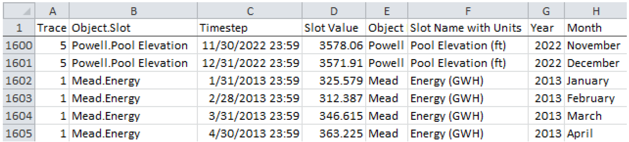
RiverWare uses end of timestep format for all datetime references. Thus for a 1 Month timestep, July 2014 would be fully specified as 7/31/2014 24:00. Tableau and Excel do not have a concept of 24:00 as a time but would instead use 8/1/2014 00:00 for the same point in time. Therefore with the proper timestep option selected in the dialog, one minute is subtracted from all timestep values (e.g. 7/31/2014 23:59) to assure that they appear with the appropriate day and month references in Excel and Tableau.

Note: If the specified CSV file already exists, the CSV output from the new MRM run will overwrite the existing CSV file. It will not append data to the existing file.

NetCDF Files

Network Common Data Format (netCDF) files can be generated from the MRM run outputs. The configuration allows for the selection of various pieces of information to be used as global attributes and slot (variable) attributes. Time and Traces are treated as dimensions.

Note: RiverWare will write the file in the netCDF-3 format, with one unlimited dimension (time). The output does not use any of the features available in netCDF-4 and testing has shown that netCDF-3 provides a much smaller file size than using netCDF-4.

1. Near the bottom of the Output tab in the MRM configuration dialog, select the checkbox for Generate NetCDF Files.

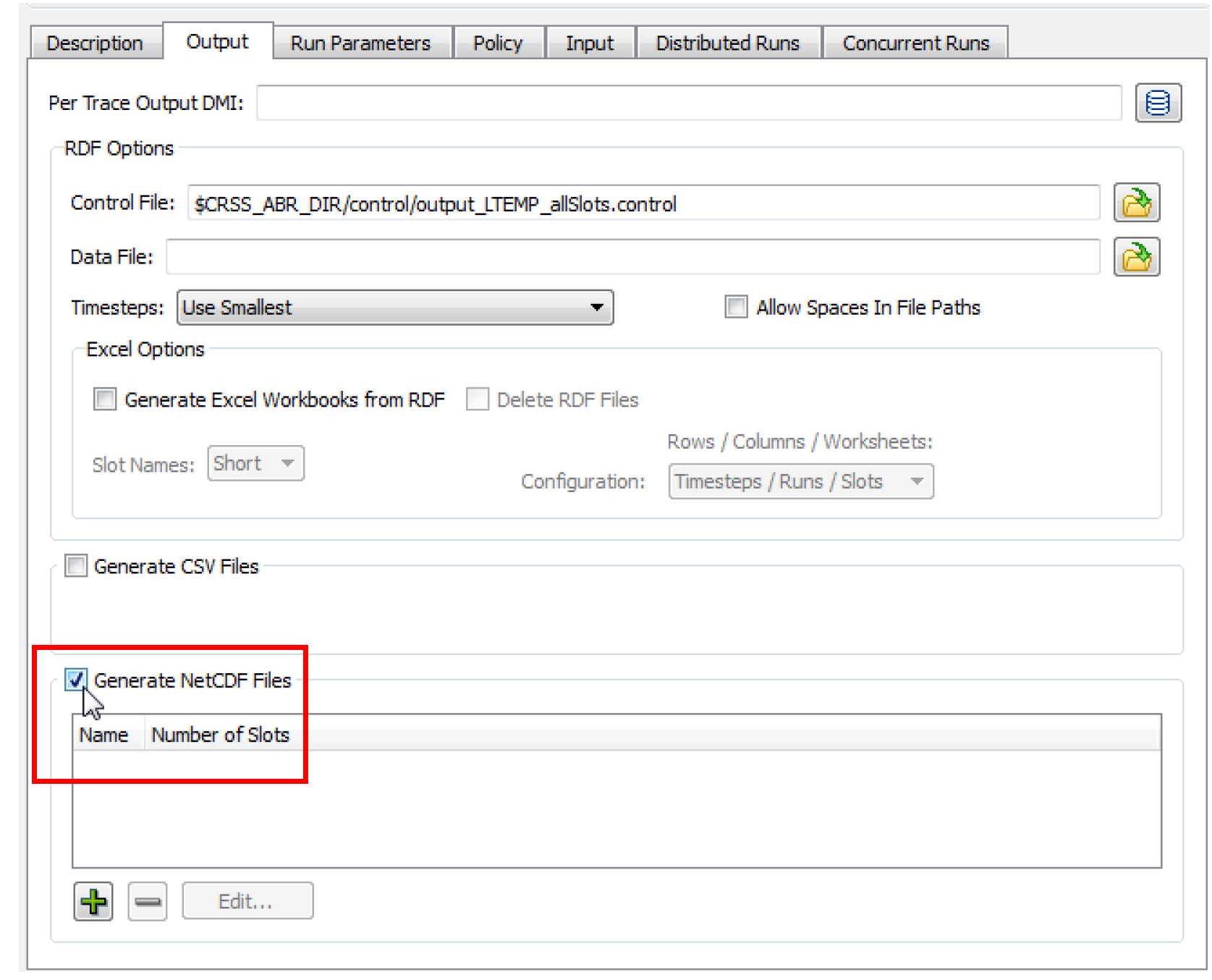
2. Select the Plus sign to add a new netCDF output file. Then select Edit to configure its contents. This will open the NetCDF File Configuration dialog.

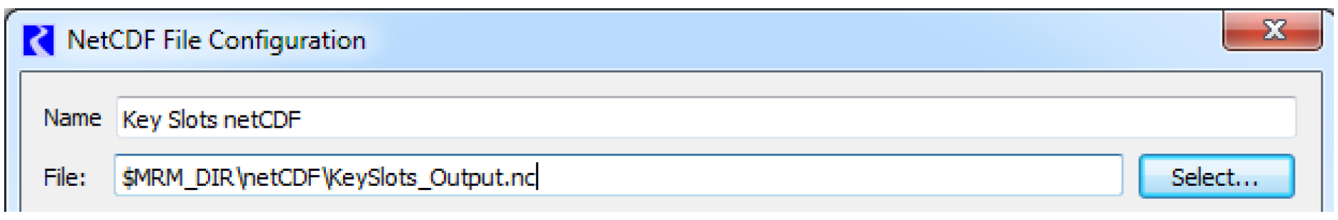
3. The netCDF file can then be given a name to display in the list in the MRM configuration.

4. In the File field, either select a netCDF file to which the new outputs should be written by selecting the Select button, or type in a complete file path. Environment variables can be used in the file path preceded by a “$”.

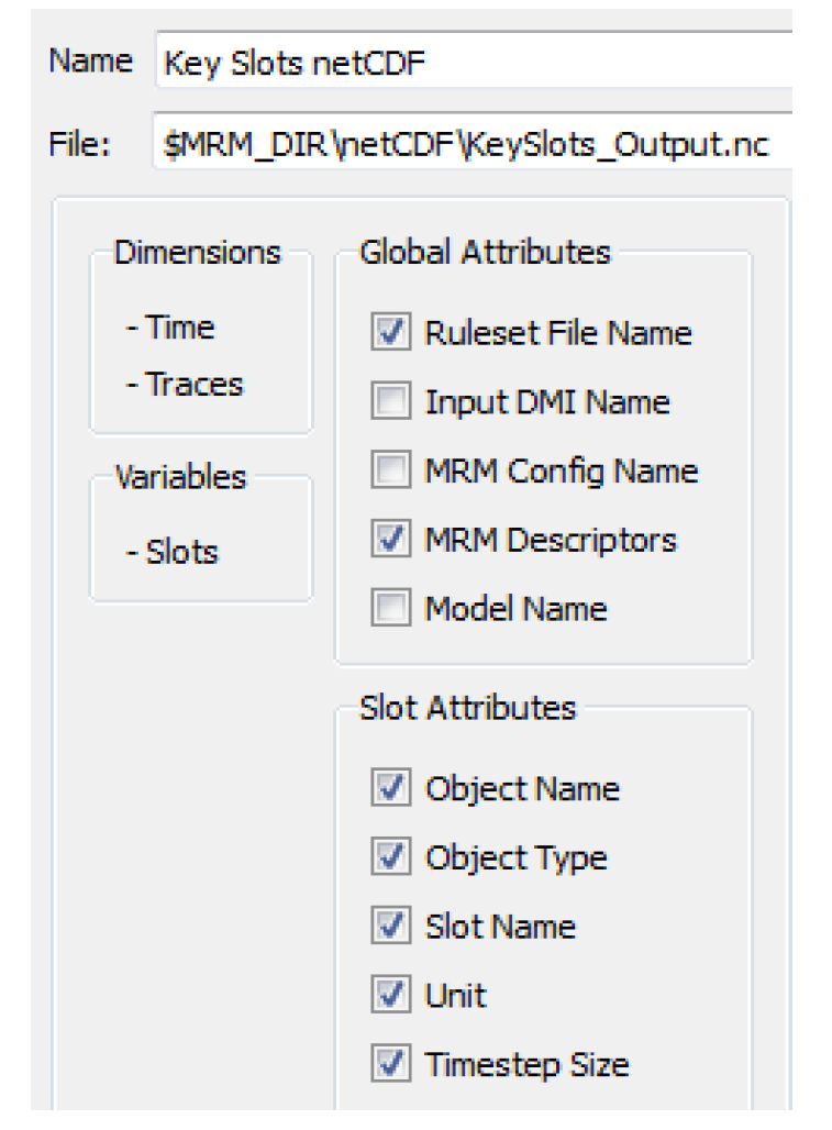
5. Next, optionally select global attributes and slot attributes to be included with the outputs by selecting or clearing the checkbox by each element.

Note: Time (timestep) and Traces (Trace Number) will automatically be used as dimensions in the netCDF output.

6. Then add slots to the netCDF output by selecting the Plus sign below the Slots panel. This will open a slot selector dialog, which can be used to add the desired slots. A slot can be removed from the selection by selecting it in the list to highlight it, then selecting the Minus sign. The Object.Slot name will be used as the variable name in the netCDF file.

7. After configuring the netCDF output, select OK in the NetCDF File Configuration dialog, and select Apply or OK in the MRM Configuration dialog to apply the changes.

Saving and Restoring Initial Model State

This section describes how to save and restore the initial state of a model. The functionality allows users to save model data to a temporary file before a multiple run is invoked and then restore this information after the run has completed.

• Open the MRM Dialog by selecting Control, then MRM Control Panel from the main RiverWare menu bar or select the MRM button on the toolbar.

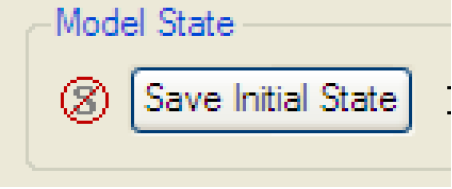
• Save the initial state of a model before invoking a MRM run by pressing the Save Initial State button in the Model State area of the MRM Control Panel.

• Start the MRM run by pressing the Start button.

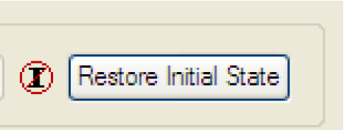
• After the run has finished, restore the initial model state by selecting the Restore Initial State button.

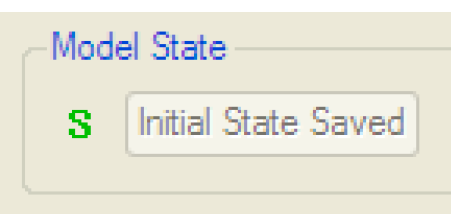
Selecting the Save Initial State button saves the entire contents of the model, including both input and output slots, TableSlots, selected user methods, run information, and configuration to a file in your temporary directory (defined by the TMP environment variable or system temporary variable as shown in the Help, then About RiverWare menu, then select the Show System Info button). Once the initial state has been saved, the button is disabled and reads “Initial State Saved.”

• Save Initial State button prior to saving state.

• Save Initial State button after saving state.

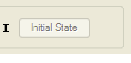
Once an initial state has been saved, it can be restored by selecting the Restore Initial State button. This reloads the entire contents of the model at the time its state was saved, clearing all data and configuration in the current state of the model. Until a multiple run has occurred, this button is disabled and reads “Initial State”.

• Restore Initial State button before a multiple run.

• Restore Initial State button after a multiple run.

Distributed Concurrent Runs

When performing concurrent MRM runs consisting of many runs, the following are some problems that users encounter:

• The memory required may exceed the resources available and/or

• The time required to make the runs is excessive.

This section describes a utility that solves these two issues by distributing many runs across many processors on the same machine.

Note: All runs are made on the same computer that has multiple cores or multiple logical processors. In this document, each separate MRM instance is referred to as a simulation processor.

In this approach, there is a controller processor and simulation processors. The controller processor does the following:

1. Creates the configurations

2. Controls execution (Start and Stop) of each simulation.

3. Tracks the progress.

4. When all the runs are finished, combines the output RDF file from each simulation into one output RDF file.

Figure 3.7

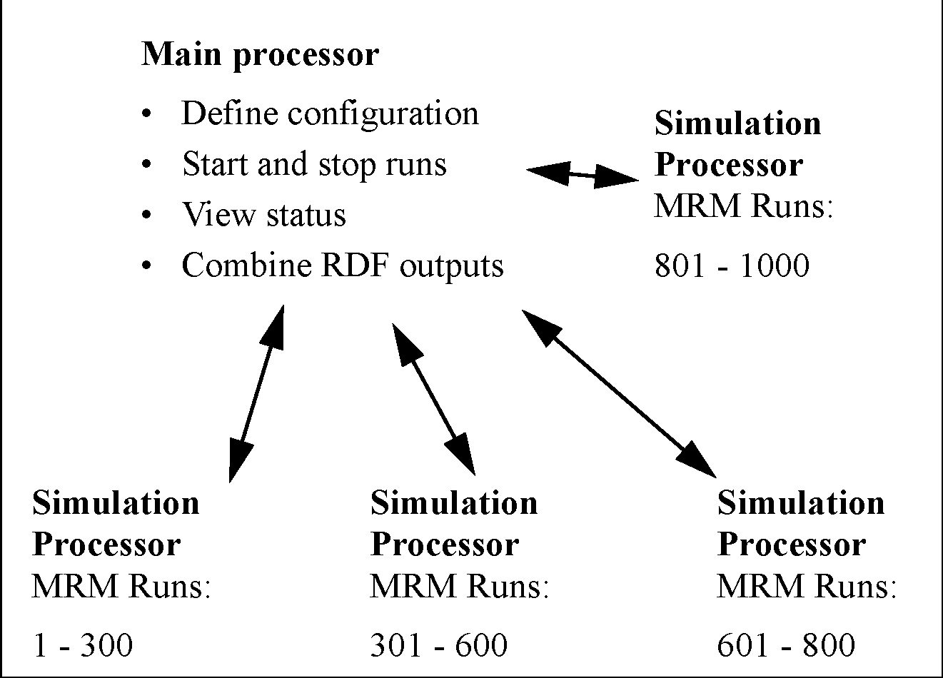
Each simulation processor then executes the MRM runs that the controller gives it to execute. Each processor runs one or more MRM runs that consist of a portion of the total number of concurrent runs. This is shown graphically in the screenshot. In this example, there are 1000 runs that are distributed unequally to four processors.

Note: If you are running RiverWare using a floating license, you can only run as many RiverWare sessions as your license allows. For example, a three-seat floating license can only run 3 RiverWare sessions. Therefore, you can distribute an MRM run to only three processors. If you wish to distribute to more processors, check out a roaming license. Node-locked and roaming licenses can run unlimited RiverWare sessions. The license guides can be found at the following URL:

http://www.riverware.org/users/

This feature was initially designed for a very specific application of concurrent MRM. As such, the following are the limitations and constraints:

• The same version of RiverWare must be used for each run.

• In the MRM configuration, the Inputs must be Traces or Index Sequential with the Pairs mode selected. See “Combined Runs” for details.

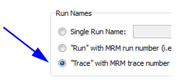
• Input DMIs can include Control File-Executable or Excel Database DMIs with the Header approach. If using Excel, you must use the Trace configuration option for the Run Names. The Run option is not supported.

Figure 3.8

• Only a single ruleset may be used.

This document is organized to present an overview of the user interface, how to make a run, and how the utility works to distribute the runs.

User Interface Overview

The interface for distributing MRM runs across multiple simulations consists of two components, the MRM configuration within RiverWare and the Distributed MRM dialog which is external to RiverWare.

MRM Configuration

MRM runs can only be distributed when in Pairs mode; see “Combined Runs”. Thus, when in Pairs mode, the Input tab has a Distributed Runs checkbox that becomes enabled. When checked, the Distributed Runs tab is added to the dialog.

As discussed in the sections that follow, the Distributed Runs tab allow you to configure:

• The working directory.

• Whether the configuration should be saved to a file.

• The number of multiple runs to distribute the traces across.

• Environment variables and their values.

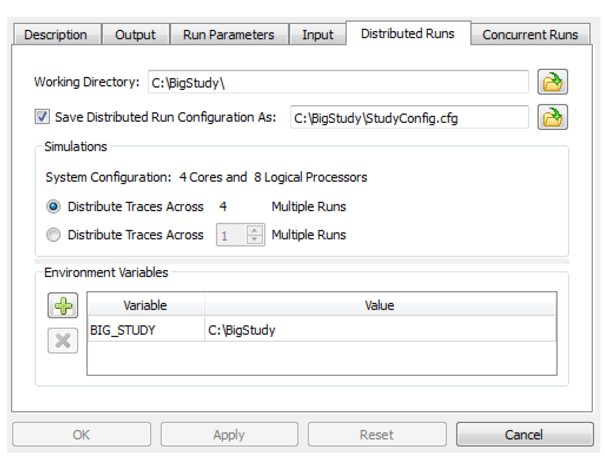
Working Directory

A distributed concurrent run creates several working files - batch script files, control files, intermediate RDF files and log files among them. The working directory specifies where the working files will be created. Importantly, it should be a directory which the controller processor and all simulation processors have access to (via the same path).

Save Configuration As

When a distributed concurrent run is started, RiverWare writes a configuration file, invokes the Remote Manager process, and exits. If a user elects to save the configuration to a named file, it is possible to invoke the Remote Manager directly bypassing RiverWare. See “Creating or Changing a Configuration” for details.

Simulations

The Simulations section defines the simulation processors and the traces they will simulate.

• System Configuration. This provides the number of cores and the number of logical processors on the machine. You can distribute your runs as follows:

• Distribute Traces across N Multiple Runs. Use all available cores on the machine. The model can be moved to different computers and the configuration will use all of the cores.

• Distribute Traces across <N> Multiple Runs. Specify the distribution. Specify a set number of runs so the runs complete in a reasonable amount of time without using all of a computer's resources. Or if you have a lot of RAM, you may specify a larger number, likely up to the number of logical processors.

The choice is ultimately hardware and model dependent. To make the best choice you will need to have detailed knowledge of your model’s memory usage and hardware. Tools like SysInternals may help to identify the maximum working set when running the model. Experimentation may be necessary to determine the most efficient settings.

Environment Variables

You can enter environment variables and value pairs.

Remote Manager and Status Dialog

As mentioned above, the Remote Manager includes a user interface which displays the status of the simulations. This dialog is not within RiverWare but is a separate executable in the installation directory. It is also opened automatically when you make a distributed MRM run from the RiverWare MRM Run Control. More specifically, the Remote Manager user interface allows you to:

• Start and stop the simulations individually or collectively.

• View RiverWare’s diagnostic output for the simulations.

• View the multiple and single run status.

• See an estimated time remaining.

• See the status of the post-processing (combining the RDF files).

In Figure 3.9, from left to right, are the Process Status, Multiple Run Status, and Single Run Status panels.

Figure 3.9

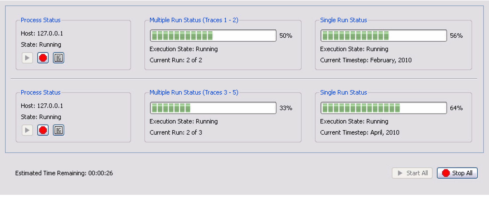
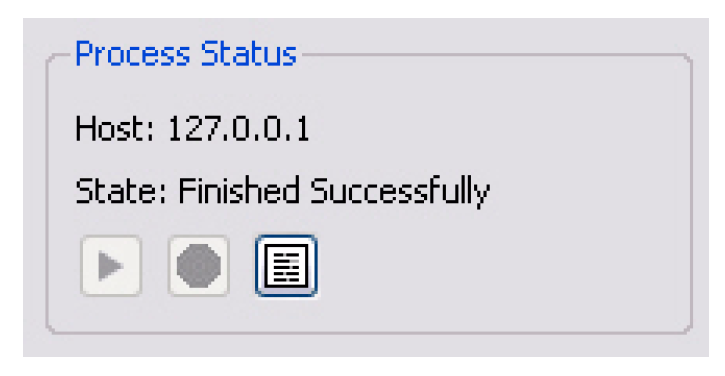
The Process Status panel includes the Start, Stop, and View Diagnostics buttons. The buttons allow you to start, stop, and view diagnostics for the individual run/process.

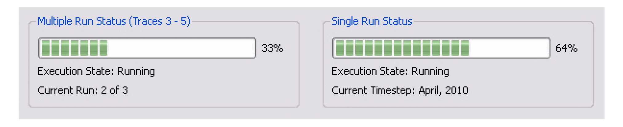
The Multiple Run Status and Single Run Status panels (which are very similar to RiverWare’s run status dialog) display the progress of each MRM run and each individual run:

The bottom of the dialog shows the estimated time remaining based on available data after the first run has completed.

How to Make a Distributed Run

There are two options, creating/changing the configuration (within RiverWare) or rerunning a configuration (can be external to RiverWare). These are described in the next two sections:

Creating or Changing a Configuration

If you are creating a new configuration or changing an existing configuration, the changes must be made from within RiverWare. This will allow RiverWare to create the necessary configuration files that will be passed to the simulation controllers. When you select Start, RiverWare will create the necessary configuration files, start the RiverWare Remote Manager, and then exit. The RiverWare Remote Manager controls the execution of the MRM runs.

Use the following steps to make the runs in this case:

1. Open RiverWare.

2. Fully define the configuration or make any changes to an existing configuration in the MRM Run Control Configuration dialog. See “User Interface Overview” for the options.

3. Apply the changes.

4. SAVE THE MODEL. The distributed runs open and run the model that is saved on the file system. Therefore, you should save the model now, so that the configuration is preserved. Any changes to the model (including external files such as the RDF control file) will invalidate the saved configuration file.

5. Select Start on the Multiple Run Control Dialog. RiverWare will start the Remote Manager and then start the shutdown sequence. It will prompt you for confirmation so you can cancel at any time.

6. From the Remote Manager, select Start to start the distributed runs. See “Remote Manager and Status Dialog” for details.

7. The individual runs start and the status is shown including an estimate of the time remaining.

8. When all runs are complete, the output RDF files are combined into one final RDF file.

Rerunning a Configuration

If you are repeating a previously saved configuration, then you can execute the RiverWare Remote Manager directly and not open the RiverWare. In that case, you start at Step 6.. The Remote Manager will first open a simple dialog allowing you to select the configuration file and will then open its user interface. See “Save Configuration As” for details.

How It Works

Figure 3.10 illustrates the distributed architecture. In the distributed architecture there is a controller processor and one or more simulation processors.

The distributed architecture includes two processes - the RiverWare Remote Manager (RwRemoteMgr.exe) and instances of RiverWare (RiverWare.exe).

Figure 3.10

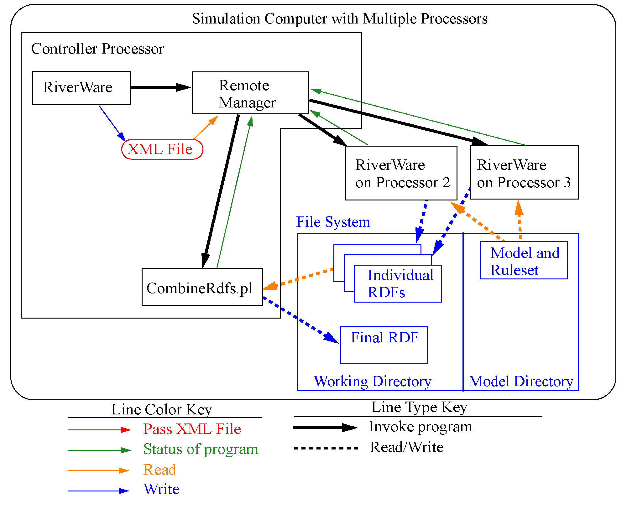
RiverWare Remote Manager

The RiverWare Remote Manager parses an XML configuration file that defines the simulations and:

• Creates an XML configuration for each of the simulations.

• Configures its user interface (a dialog which shows the status of the simulations).

• For each simulation, connects to the simulation processor, writes the XML configuration, and reads RiverWare’s output (which it uses to update its status dialog).

• When all simulations have finished, combines the partial RDF files to create the final RDF files.

XML Configurations

Previous sections have referred to XML configurations. These are the files that RiverWare creates to control/define the distributed MRM runs.

Note: This section is a technical reference providing more information on how this utility works. The XML files are generated by the utility and the user does not need to edit these files to make a distributed MRM run.

The top-level XML configuration <distrib> identifies a distributed concurrent run and is hereafter referred to as the distributed configuration. An XML document defining a distributed concurrent run would have the following top-level elements:

...

</distrbv>

</document>

The XML document defining a distributed concurrent run is created by RiverWare when a user starts the run. DistribMrmCtlr parses the distributed configuration and creates a configuration for each of the simulations. Some elements are from the MRM configuration, others are provided by RiverWare. Some elements are common to all simulations, others are unique to each simulation.

Example 3.1 Sample XML File

Key elements in this example are preceded by brief descriptions.

The RiverWare executable which started the distributed concurrent run. The assumption is that all simulations use the same executable.

<app>C:\Program Files\CADSWES\RiverWare 6.4\riverware.exe</app>

The model loaded when the user starts the distributed concurrent run.

<model>R:\\CRSS\\model\\CRSS.mdl</model>

The global function sets loaded when the user starts the distributed concurrent run.

<gfs>R:\\CRSS\\model\\CRSS.gfs</gfs>

</gfslist>

The config attribute is the MRM configuration selected when the user starts the distributed concurrent run. The mrm elements are from the MRM configuration and identify for each simulation the traces to simulate.

</mrmlist>

The rdflist element is a list of the final RDF files, while the slotlist element is a list of the slots which are written to the RDF files. Slots can be written to multiple RDF files; they’re associated with the RDF files by the idxlist attribute, whose value is a comma-separated list of RDF file indices. RiverWare initializes the RDF DMI and mines its data structures to generate rdflist and slotlist.

</rdflist>

</slotlist>

The envlist element specifies RiverWare’s runtime environment; RIVERWARE_HOME is from the version of RiverWare which starts the distributed concurrent run, all others are from the MRM configuration.

<env>RIVERWARE_HOME_516=C:\\Program Files\\CADSWES\\RiverWare 5.1.6 Patch</env>

</envlist>

The tempdir element is from the MRM configuration and is the intermediate directory where the individual simulations write the partial RDF files.

</distrib>

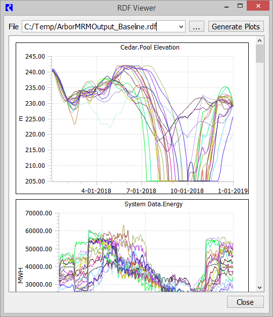
RDF Viewer

The RDF Viewer is a simple tool for quickly visualizing the RDF results of an MRM run. A sample RDF file is shown as over plotted lines in Figure 3.11. This section describes the RDF Viewer and how to use it.

Figure 3.11 Screenshot of the RDF Viewer

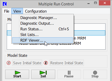
Accessing the RDF Viewer

Access the RDF Viewer from the Multiple Run Control dialog using the View and then RDF Viewer menu as shown in Figure 3.12.

Figure 3.12 Multiple Run Control with RDF Viewer menu

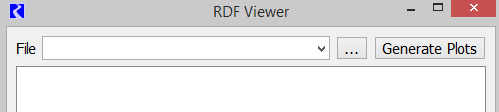
Then the RDF Viewer opens as shown in Figure 3.13.

Figure 3.13 RDF Viewer with no file specified

How to Use the RDF Viewer

Within the RDF Viewer, type a file path and name or use the ellipsis button to open a file chooser, then select the desired RDF file and click Open. The RDF Viewer will read the RDF file and automatically generate plots of the slots. The tool displays plots of the RDF data, one plot per slot, with runs (traces) over plotted as shown in Figure 3.11

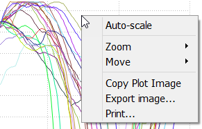
Hover over a curve to see the run/trace number. Right click on a plot area for additional plotting functionality as shown in Figure 3.14. In addition, use the mouse wheel to zoom in/out on either the plot area or the axis. Click and drag the middle mouse button to pan the plot.

Figure 3.14 RDF Viewer Plotting controls.

Revised: 11/11/2019