
Hydrology Simulator Event
The Hydrology Simulator event takes observed annual streamflow values and synthesizes an ensemble of annual flow data for a user-specified number of traces. These trace flow files can then be imported through a DMI to a RiverWare multiple run.
Note: For the Hydrology Simulator to successfully generate hydrology ensembles, the R Project for Statistical Computing must be installed on your computer; see Install R and Component Packages for details. This event was developed and tested with R version 2.14.2, but it should work with newer versions of R.
Note: The Hydrology Simulator should be used for annual flow data only. The event does not have any knowledge of the timestep size and will technically simulate with flow data based on any timestep. However, the algorithm does not have any means to account for seasonality, and thus, the results are only meaningful for annual data. For details and disaggregating annual flow data to monthly, see Temporal Disaggregation Event.
Available Functions
The Hydrology Simulator provides the following functions for generating ensembles.
Resampled KNN
This function resamples historic streamflow values using the k-Nearest Neighbor algorithm; see Resampled KNN Function Configuration for configuration details. The general algorithm is as follows.
1. For the first simulated year, a year is selected randomly from the historic streamflow data. For all subsequent years in the Trace Length, the following steps are carried out.
2. The historic years are sorted based on the difference in their flow relative to the flow of the previous simulated year to find the “nearest neighbors.”
3. The k number of “nearest neighbors” are selected. The k value is the square root of the number of values in the historic streamflow time series.
4. The nearest neighbor years are weighted with the highest weight on the year most similar to the previous simulated year.
5. A sample is taken from the nearest neighbor years based on the weighting.
6. The year following the selected year in the historic streamflow sequence is taken as the simulated flow on the current timestep.
Paleo Conditioned Homogeneous Markov Chain
This function resamples historic streamflow values using paleo-reconstructed streamflow sequences; see Paleo Conditioned Homogeneous Markov Chain Interface Function Configuration for configuration details. The general algorithm is as follows.
1. The historic streamflow data are divided into two transitional states (wet and dry) or three transitional states (very wet, normal, and very dry), as specified by the user.
2. A transition probability matrix, which represents the probability of each of the states occurring on a given year given the state the previous year, is created from the entire paleo period.
3. For the first simulated year, a year is selected randomly from the historic streamflow data. For all subsequent years in the Trace Length, the following steps are carried out.
4. Given the state from the previous timestep, and using the transition probabilities as weights, a state is selected for the current timestep.
5. An observed streamflow value from the selected state is chosen using the k-Nearest Neighbor algorithm.
Paleo Conditioned Nonhomogeneous Markov Chain
This function resamples historic streamflow values using paleo-reconstructed streamflow sequences; see Paleo Conditioned Nonhomogeneous Markov Chain Interface Function Configuration for configuration details. The general algorithm is as follows.
1. The historic streamflow data is divided into two transitional states (wet and dry) or three transitional states (very wet, normal, and very dry), as specified by the user.
2. A transition probability matrix, which represents the probability of each of the states occurring on a given year given the state the previous year, is created from a randomly selected window from the paleo period of length equal to Trace Length; this is what differentiates this method from the Homogeneous Markov Chain method, which uses the entire paleo record to establish th transition probabilities.
3. For the first simulated year, a year is selected randomly from the historic streamflow data. For all subsequent years in the Trace Length, the following steps are carried out.
4. Given the state from the previous timestep, and using the transition probabilities as weights, a state is selected for the current timestep.
5. An observed streamflow value from the selected state is chosen using the k-Nearest Neighbor algorithm.
Hydrology Simulator Configuration Dialog Box
This dialog box opens when you open a Hydrology Simulator event on the RiverSMART workspace.
Name
Enter a unique user-defined name for the Hydrology Simulator event.
Function
Select the hydrology function to use, as follows.
• Resampled KNN; see Resampled KNN Function Configuration for details.
• Paleo Conditioned Homogeneous Markov Chain; Paleo Conditioned Homogeneous Markov Chain Interface Function Configuration for details.
• Paleo Conditioned Nonhomogeneous Markov Chain; Paleo Conditioned Nonhomogeneous Markov Chain Interface Function Configuration; for details.
Resampled KNN Function Configuration
If you select the Resampled KNN option in the Function field, the Hydrology Simulator Configuration dialog box appears as follows.
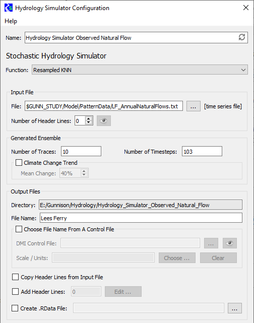
Input File frame
In this frame, you specify information about the input file, which is a single time series of observed historic flows for the desired site.
File
Specify the input file to use. You can enter the path or select it through the File Chooser.
Number of Header Lines
Enter the number of non-data header lines in the input file. The R scripts expect the file to start with data values; therefore, if there are header lines, this entry is required to inform the scripts how many lines to skip. If you need to see how many header lines there are, select Preview to preview the file in a separate window.
Generated Ensemble frame
In this frame, you specify information to configure the generated ensembles.
Number of Traces
Enter the number of traces in the ensemble.
Number of Traces
Enter the number of timesteps in each trace.
Climate Change Trend
Select the check box to apply a percentage change to the timestep values, and enter the percentage in the text box. Your entry must be a whole number, either positive or negative. Over the course of all timesteps in the trace, the values will trend linearly up or down by this percentage. The climate change trend is applied after the k-NN resampling algorithm.
Clear the check box to use the timestep values with no trend change.
Output Files frame
In this frame, you specify information to configure the output generated by the event.
Directory
Display only. displays the output folder to be created by RiverSMART. This folder is located under the Hydrology subfolder of the study folder and is named with the user-defined event name. A folder for each trace, named trace1, trace2, and so on, is created under the output folder.
File Name
Enter the file name for the resulting output file generated in each trace folder. This is typically the site name. Optionally, you can select the name from a RiverWare DMI Control File using the DMI Control File and Choose options.
DMI Control File
Select the check box to select the output file name from a DMI Control File, and specify the control file to use. You can enter the file path in the text box or select it through the File Chooser. If you need to view the file contents, select Preview to preview the file in a separate window.
Optionally, select Choose to display a list of the slot names in the specified DMI Control File. You can then select a slot, which is entered in the File Name field.
Scale/Units
Display only. Displays the units for the specified slot from the control file, if available. This is informational only and has no impact on the ensemble calculations.
Select Clear to clear the File Name and Scale/Units entries.
Copy Header Lines from Input File
Select this check box to copy the header lines in the input traces to the output files.
Add Header Lines
Select this check box to enter additional header lines to add to the output files. Select Edit, then enter the lines in the Additional Meta Data Lines dialog box and select OK when done. The number of additional lines is displayed in the text box.
Create .R Data File
Select this check box to save the R session that generates the ensembles to a file, which can be reopened later in the R application. You can enter the file path in the text box or select it through the File Chooser.
Paleo Conditioned Homogeneous Markov Chain Interface Function Configuration
If you select the Paleo Conditioned Homogeneous Markov Chain option in the Function field, the Hydrology Simulator Configuration dialog box appears as follows.
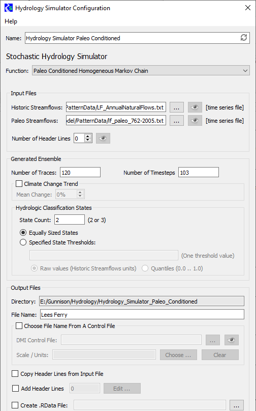
Input Files frame
In this frame, you specify information about the input files.
Historic Streamflows
These are a single time series of observed historic flows for the selected site. Specify the file with the streamflows to use. You can enter the path or select it through the File Chooser. Select Preview to preview the file in a separate window.
Paleo Streamflows
These are a single time series of paleo-reconstructed streamflows for the selected site. Specify the file with the streamflows to use. You can enter the path or select it through the File Chooser. Select Preview to preview the file in a separate window.
Number of Header Lines
Enter the number of non-data header lines in the input file. The R scripts expect the file to start with data values; therefore, if there are header lines, this entry is required to inform the scripts how many lines to skip. If you need to see how many header lines there are, select Preview to preview the file in a separate window.
Generated Ensemble frame
In this frame you specify information to configure ensembles.
Number of Traces
Enter the number of traces in the ensemble.
Number of Traces
Enter the number of timesteps in each trace.
Climate Change Trend
Select the check box to apply a percentage change to the timestep values, and enter the percentage in the text box. Your entry must be a whole number, either positive or negative. Over the course of all timesteps in the trace, the values will trend linearly up or down by this percentage. The climate change trend is applied after the k-NN resampling algorithm.
Clear the check box to use the timestep values with no trend change.
Hydrologic Classification States frame
In this frame, you enter information defining the hydrologic states used in the calculations.
State Count
Enter the value classifying the hydrology for each year; valid entries are as follows:
• 2 = dry/wet
• 3 = very dry/normal/very wet
Equally Sized States
Select this option to size the states equally.
Specified State Thresholds
Select this option to size the states according to user-defined settings. Enter the threshold values in the text box. If the State Count is 2, enter one threshold value; if the State Count is 3, enter two values, separated with a comma.
Select one of the following options to specify the type of values used to define the thresholds.
• Raw values (Historic Streamflows units). Select this option if the threshold values represent raw flow values.
• Quantiles (0.0 .. 1.0). Select this option if the threshold values represent quantiles; valid entries are 0.0–1.0.
Output Files frame
In this frame, you specify information to configure the output generated by the event.
Directory
Display only. displays the output folder to be created by RiverSMART. This folder is located under the Hydrology subfolder of the study folder and is named with the user-defined event name. A folder for each trace, named trace1, trace2, and so on, is created under the output folder.
File Name
Enter the file name for the resulting output file generated in each trace folder. This is typically the site name. Optionally, you can select the name from a RiverWare DMI Control File using the DMI Control File and Choose options.
DMI Control File
Select the check box to select the output file name from a DMI Control File, and specify the control file to use. You can enter the file path in the text box or select it through the File Chooser. If you need to view the file contents, select Preview to preview the file in a separate window.
Optionally, select Choose to display a list of the slot names in the specified DMI Control File. You can then select a slot, which is entered in the File Name field.
Scale/Units
Display only. Displays the units for the specified slot from the control file, if available. This is informational only and has no impact on the ensemble calculations.
Select Clear to clear the File Name and Scale/Units entries.
Copy Header Lines from Input File
Select this check box to copy the header lines in the input traces to the output files.
Add Header Lines
Select this check box to enter additional header lines to add to the output files. Select Edit, then enter the lines in the Additional Meta Data Lines dialog box and select OK when done. The number of additional lines is displayed in the text box.
Create .R Data File
Select this check box to save the R session that generates the ensembles to a file, which can be reopened later in the R application. You can enter the file path in the text box or select it through the File Chooser.
Paleo Conditioned Nonhomogeneous Markov Chain Interface Function Configuration
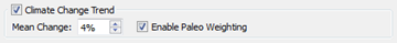
If you select the Paleo Conditioned Nonhomogeneous Markov Chain option in the Function field, the Hydrology Simulator Configuration dialog box appears the same as for the Paleo Conditioned Homogeneous Markov Chain function, with the addition of the following check box in the Generated Ensemble frame.
Enable Paleo Weighting
Select this check box to enable paleo weighting for the climate change calculation.
See Paleo Conditioned Homogeneous Markov Chain Interface Function Configuration for details about the remaining fields.
Revised: 08/02/2021