
Types of Slots
This section presents a description of the different types of slots and how they are used for representing different types of data. Select a link for full details on how to view, create, and edit that type of slot.
Name | Icon | Type | Description |
|---|---|---|---|
Series Slot |  | Series | A single timeseries of values. These slots may be linked with another Series Slot. Input data in Series Slots controls the simulation solution, and all simulation output data are written to Series Slots. Custom slots can be linked to any linkable slot on the workspace. |
Series Slot with Expression |  | Series | A specialized Series Slot whose value is computed from a user-defined arithmetic expression possibly containing other slot names as variables. They are used to calculate quantities such as “combined Storage of all Reservoirs.” |
Text Series Slot |  | Series | A specialized Series Slot whose values are text strings instead of numerical data. They are used to store annotations or strings. |
Integer Indexed Series Slot |  | Series | A specialized series slot that is indexed by an integer number instead of a date. |
Agg Series Slot |  | Series | A specialized Series Slot that is an aggregation of one or more Series Slots which are independent of one another. They are used to group together similar series of data. |
Integer Indexed Agg Series Slot |  | Series | An Agg series slot that is indexed by an integer number instead of a date. |
Series Slot with Periodic Input |  | Series | A Series Slot with Periodic Input is technically a series slot, but you can optionally input data in the same format as a periodic slot. When entered periodically, the slot automatically fills out the series values. |
Multi Slot |  | Series | A specialized Series Slot aggregating one or more Series Slots. The value in the first Series Slot column is the sum of the values in all of the other Series Slot columns (other slots to which they are linked). New Series Slot columns are automatically added when a link is made to the Multi Slot. |
Table Slot |  | Table | A two or three-dimensional table of values for representing one or more functional relationships. Each column stores a variable with its own unit type and name. Rows are numbered beginning with 0. Both rows and columns can be referenced by using an index (0, 1, 2 . . . n) or using a label string. For a three-dimensional table lookup to be successful, column 1 must contain blocks of equal values which increase down the table, and column 2 must contain monotonically increasing values within each block of values from column 1. A two-dimensional table only requires monotonically increasing values in its first column. Table functionality includes accessing values beginning with the table indexes and accessing a column index beginning with row index and table value. |
Statistical Table Slot |  | Table | A specialized table slot allowing the user to specify a statistical function, such as flow duration curve, which is computed at the end of a run using the data in specified model slot(s). This statistical analysis data can then be plotted or exported. |
Table Series Slot |  | Table | A specialized table slot whose rows correspond to time values. This slot contains limited timeseries functionality thus making it more efficient, performance wise than Series Slots. It is commonly used for writing and reading large amounts of data. It is primarily used within user methods; you cannot create them as custom slots. |
Periodic Slot |  | Table | A specialized table slot, the periodic slot is used to hold data that repeats over a specified time period. For example, a set of monthly evaporation coefficients for a reservoir (the same every year), could be held in a periodic slot. The timeseries associated with the data can vary (1 Hour, 1 Day, 1 Month, etc.) as well as the period over which the data repeats. The periodic slot can also handle irregular timeseries and can have either text or numeric column headings. |
Scalar Slot |  | Scalar | The scalar slot is used to hold a single piece of numeric data that will not vary with time. |
Scalar Slot with Expression |  | Scalar | A scalar slot whose value is computed from a user-defined arithmetic expression. The expression can contain values from other slots as variables. |
Mass Balance Summary |  | Mass Balance Summary | The mass balance summary slot is a user-defined hierarchy of series slot collections used to check mass balance across many objects. |
Time Aggregation Series Slots |  | Series | Time Aggregation Series Slots temporally aggregate any other single series slot. It can be recomputed manually or automatically at the end of a run. |
Time Disaggregation Series Slots |  | Series | Time Disaggregation Series Slots temporally disaggregate any other single series slot using either a step or interpolation function. It can be recomputed manually or automatically at the end of a run. |
List Slot |  | List | The list slot is used in certain user methods to specify a list of objects or slots associated with that method. The user cannot add custom List Slots. |
Series Slots
There are several types of time series slots with various column configurations. Since all of these slot types contain rows that correspond to the series of data, they will be referred to collectively as series slots. Most series slots open automatically in a Slot Viewer. Any slot shown in the viewer can be detached from the viewer and shown in its own Slot dialog by dragging the column off the viewer.
Slot Dialog and Slot Viewer
Figure 5.7 highlights the differences between the individual Slot dialog and the Slot Viewer.
Figure 5.7 Screenshot comparing a Slot Dialog and the Slot Viewer
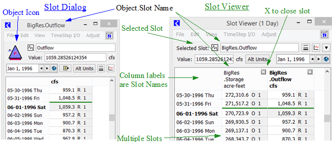
How many of each dialog are there?
There is one Slot Viewer for each timestep (1 Day, 1 Month, and so on) per model. There can be many Slot dialogs.
What types of slots are shown?
There is a Slot dialog for each type of slot. The Slot Viewers show series slots.
Which slots will open in the Slot Viewer?
Series slots, Text Series slots, Series Slots with Periodic Input, and Multi slots with a single subslot open automatically in the Slot Viewer. Multi slots with two or more subslots and Expression slots open in their own Slot dialog but can be docked in the Slot Viewer.
Agg Series slots with two or more columns will be shown in their own slot dialog. Scalar slots will open in their own Slot Viewer. See Scalar Slot Dialog and Slot Viewer (Scalar) for more information.
All other types of slots (Periodic, Table) are shown in their own Slot dialog.
How do I get back to the slot viewer if it gets minimized or hidden?
The workspace has a Slot Viewers button in the lower right. This shows the selected Slot Viewer when it has been minimized or hidden behind other dialogs. Remember, if the Slot Viewers have been closed or all slots are removed from it, the Slot Viewers are longer exists and the button is disabled.
Can the two types of dialogs interact?
From the Slot Viewer, you can drag a slot off of the viewer to become a single Slot dialog. You can then drag the slot icon on the series slot and drop it on the Slot Viewer to redock it. The Slot Viewer must have the same timestep size as the slot. See Slot Viewer Functionality for details.
Where can I find more information?
Slot Viewer Functionality
The Slot Viewer is an ad hoc tool to view multiple series slots in a single dialog. There is one Slot Viewer per timestep size in a RiverWare session. The slots shown and order is not persistent in any way on the viewer. Each time a Series Slot is opened from anywhere in RiverWare, it is added as a column to the Slot Viewer. From the Slot Viewer, any slot can be shown also in the slot's conventional Slot dialog.
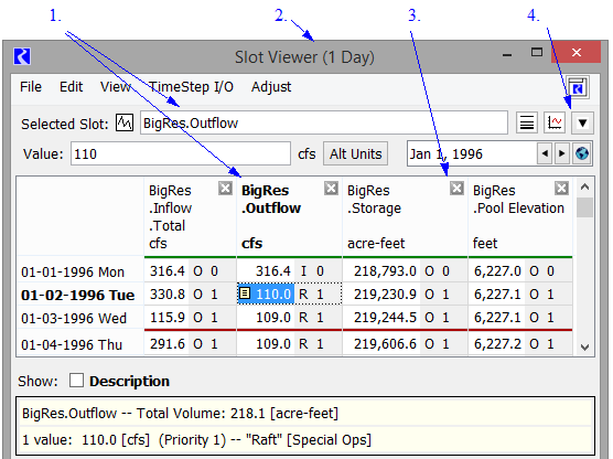
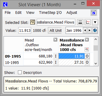
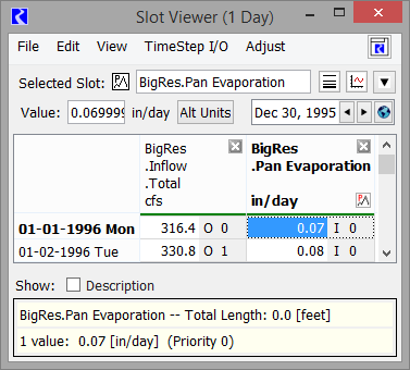
Figure 5.8 shows the Slot Viewer showing four slots on BigRes. The annotations correspond to the following numbers:
1. Selected Slot
2. Slot Viewer Timestep Size
3. Close Slot
4. List of Slots in the Viewer
The Slot Viewer shows different menu options based on the selected slot. Highlight cells in a single column (or the entire column) to select a slot. If you highlight cells in multiple columns, the Selected Slot is blank and many of the menu options are disabled. For certain types of slots, like expression slots and Series Slots with Periodic Input, not all of the menu options are shown on the slot viewer. Undock the slot and use the Slot Dialog to access all of the configuration and menu options.
Figure 5.8 Screenshot of a Slot Viewer with annotations described above.
Following are the Slot Viewer specific actions:
• Rearrange Columns. Drag a column header to rearrange columns.
• Undock a single slot:
– Drag a column off of the Viewer to show the slot in its own dialog.
– Right-click the column header and choose Show In Slot Dialog.
– Use the File, then Undock Selected Slot(s) menu.
• Undock all Slots. Use the File, then Undock All Slots to show all of the slots in their own dialog.
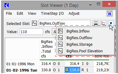
• Navigate to a slot. Use the scroll bars to scroll left/right to find the slot or use the down arrow menu to list all of the slots in the viewer. Select the desired slot to select and scroll to that slot.
• Close Slots
– Select the X at the top right of the slot column.
– Select one or more slots. Then use the File, then Remove Selected Slot(s) menu.
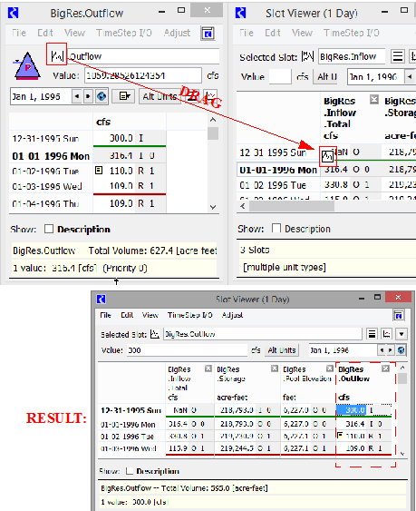
To dock a slot onto a Slot Viewer, drag the slot’s icon anywhere on the viewer. Figure 5.9 shows the icon that you should drag and the result. Alternatively, use the File, then Dock in Slot Viewer menu.
The two following types of slots have additional configuration options in the Slot Dialogs and have an additional icon/button in the column heading. Click this icon to open the slot in its own dialog and edit the periodic values.
• Series Slot with Expression show the  in the column heading. See Series Slots With Expression for more information.
in the column heading. See Series Slots With Expression for more information.• Series Slot with Periodic Input show the  in the column heading. See Series Slots With Periodic Input for more information.
in the column heading. See Series Slots With Periodic Input for more information.Figure 5.9 Screenshot showing dragging a slot onto the Slot Viewer
Series Slot Dialog Functionality
Figure 5.10 shows the key areas of a series slot. There is a DateTime selector and scroll button used to scroll to the given date. Icons and buttons are used to show display compression, show notes, and to Plot the slot. The DateTimes are shown as the row headings, the data values are shown in the cells, and each cell’s value has a flag. Bold, green separators are automatically created based on the timestep of the slot. For example, in a slot with a 1 Day timestep, separators are placed between months. In 6 Hour slot, days are separated. Also, there is a blue divider between the initial and start timestep. There is a red divider after the finish timestep.
Figure 5.10 Annotated Screenshot of a Series Slot dialog
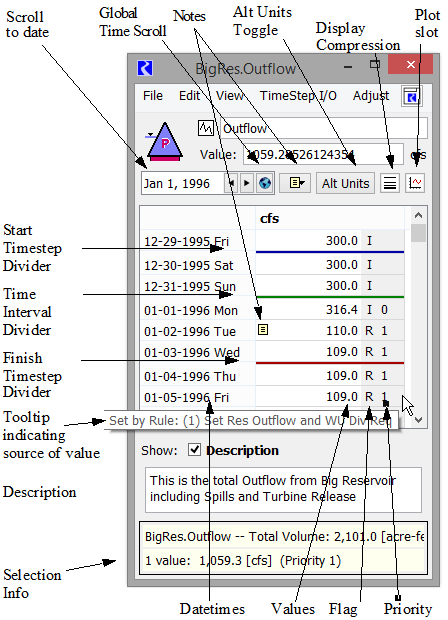
Data
Time series data are displayed with one value per row where each row represents a timestep. A scroll bar along the right side of the field is used to view the entire set of data. Each row contains the full date and time, a status flag, and the slot value at that time. A slot value which shows NaN (Not a Number) represents an unsolved variable.
The values that appear in the Open Slot dialog use the Units for that slot. See Standard Units for details on Units. See Configure Slot Dialog for details on configuring slot units.
Timesteps
Timesteps are reported chronologically. If the series is an Integer Indexed series, the rows are indexed by an integer number instead of a timestep.
Editing Slot Values
Conventional editing commands are available for all slots. They allow cutting, pasting, filling and clearing of data.
A Delete or Cut of any timestep except the first shifts data up to replace the lost cell, reassigning values to new timesteps. A Delete or Cut of the first timestep removes it completely from the series, essentially shifting the start date of the series.
Similarly, Insert New Cell or Insert Copied Cells when the first timestep is selected adds a new timestep to the beginning of the series. When any other timestep is selected, Insert New Cell or Insert Copied Cells shifts data down from the added cell, reassigning values to new timesteps.
Priority
In a Rulebased Simulation run, the dialog shows the priority of the slot at the given timestep. This can enable/disabled using the View, then Show Priorities menu.
Alt Units button
On series slots, an Alt Units toggle button  is shown in the tool bar when the slot displays any of the following:
is shown in the tool bar when the slot displays any of the following:– A slot with flow unit type
– A slot with volume unit type for certain simulation slots, like reservoir Evaporation
– A custom slot with volume unit type, and configured to show the toggle, as described in Configure Slot Dialog Functionality.
Note: This button is also shown on the Slot Viewer when there is at least one slot that meets these criteria.
Figure 5.11 Screenshot of the Alt Units options.
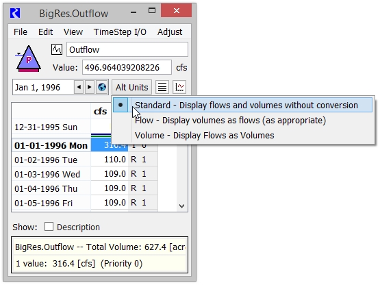
As shown in Figure 5.11, the button switches the display between
– Standard - Display flows and volumes without conversion
– Flow - Display flow slots as flows and display volumes as flows (as appropriate)
– Volume - Display flow slots as Volumes and display volume slots as volumes.
When a slot is shown with its non-default unit type, an asterisk is shown in the column label as shown in Figure 5.12.
Figure 5.12 Screenshot of flow slot showing values as Volumes. Notice the asterisk by the unit.
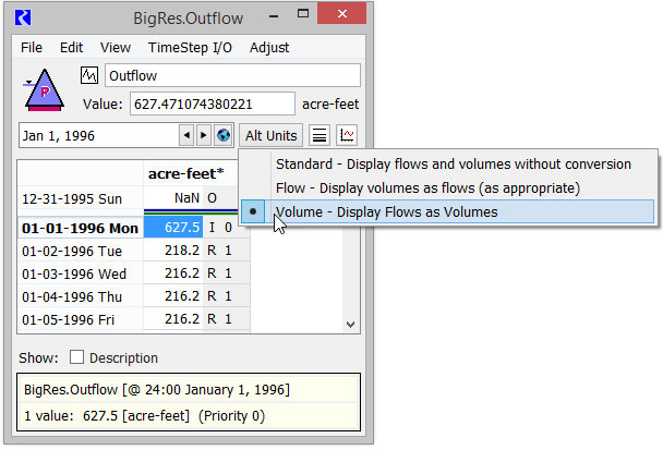
The units for both the default and alternative units are defined by the unit scheme. The unit type will apply unless an exception has been created for the slot. Exceptions can be created for both flows and volume unit types for a particular slot.
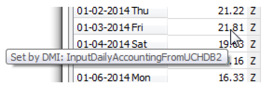
Tooltips
Tooltips provide additional information about individual values. In particular, when you hover over a value for which the relevant information is available, one of the following tooltips is displayed:
• Set by DMI. Displayed when the value was set by an input DMI that was configured to record invocations. For example, “Set by DMI: Import Lake Levels”. See DMI Invocation Manager Dialog in Data Management Interface (DMI) for details on Invocation Records.
• Set by Initialization Rule. Displayed when the value was set by an Initialization Rule. For example, “Set by Initialization Rule. (3) Provide Default Hydrology”.
• Set by Rule. Displayed when the value was set by a rule. For example, “Set by Rule: (18) Long Lake Fishery Releases”.
• Rule. Displayed when the value was solved for as a result of a rule setting a value elsewhere in the system. That is, the value was set during dispatching because a rule set a value somewhere. In this situation, the value has the output flag and the controller's priority which is also the priority of the rule whose execution triggered dispatching. For example, “Rule: (18) Long Lake Fishery Releases”.
For the last three items you can quickly open the rule associated with the value. Right-click and choose to Open Rule N from the menu.
Additional information may be shown in the tooltips when an optimization run has been made. Examples of the information are: “Frozen at Lower Bound”, or “Frozen by (3) Minimum Load 47.6% between limits set by 3.1.1.1 and 2.1.1.1.” or “Frozen by (2) Ending Pool Elevation at a limit set by 2.1.1.1”. See Tooltips on Variables in Optimization for details.
Selection Info Area
Optionally, the Selection Info Area (also called the Summary Area or Selection Statistics) can be shown using the View, then Show Selection Statistics. This displays information on the selected cells in the Slot including the name or number of slots and then statistics on the selection. Statistics include Sum, Average, Median, Min, Max, Range, and Difference. All, some or none of these may be shown depending on the number of cells selected and the units of those cells. If a single value is selected and that value was solved for or set as a result of a rule in rulebased simulation, the Priority is also shown. Finally, if the values have units of flow, power, or velocity, the selection area also shows the integrated values over time, thus showing the total volume, energy, or length, respectively. The unit scheme units for that unit type are used.
Note: You can configure your preferences on whether or not to show Selection Statistics using Slot Dialog Display Preferences; see Slot Dialog Display Preferences.
Global Time Scroll
Use the global time scroll button or the right-click context menu to change all date-based dialogs to the selected date. This date is then used for any currently opened dialogs and any that are opened from this point forward.
Configure Slot Dialog Functionality
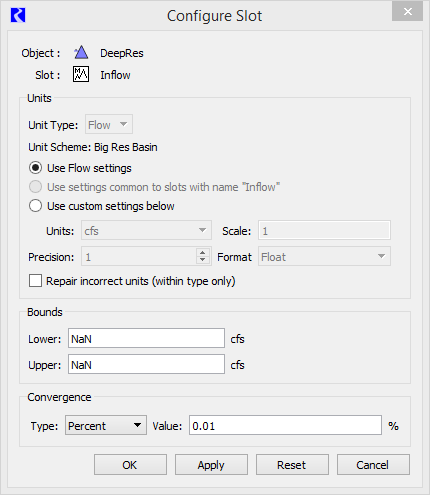
The Configure Slot dialog, shown in Figure 5.13, is displayed by selecting View, then Configure. Following are configuration options specific to Series Slots. See Configure Slot Dialog for details on general configuration.
Figure 5.13 Screenshot of the Configure Slots dialog for a series slot
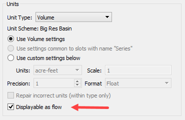
Displayable as Flow Checkbox
As described in Alt Units button, flows slots can always be shown as the volume over the timestep. But only certain simulation slots, with the volume unit, can be shown as flows, like evaporation volume. For custom slots that you create, you can choose for each volume slot whether the Alt Units will apply. When the Unit Type is Volume, the Displayable as flow checkbox is shown as noted in Figure 5.14. Check the box indicating this volume can be shown as a flow, using the Alt Units button. Leave it unchecked if the volume is not displayable as a flow.
Figure 5.14 Screenshot of Slot Configuration with Displayable as flow setting
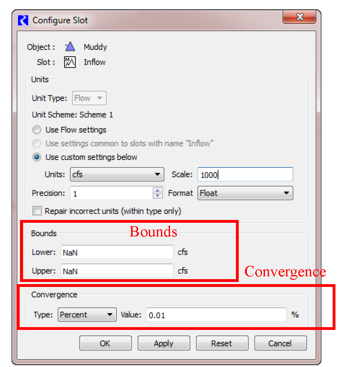
Setting Bounds on a Series Slot
Series slots have upper and lower bounds as shown in Figure 5.15. In general, these values are not used by the simulation but are used in optimization. However, there are a few cases where a value can be used by the Object’s user methods. For example, the lower bound on Outflow on a Reach object is used to calculate the maximum allowable diversion. If no value is specified, the total Inflow may be diverted.
Figure 5.15 Screenshot of the Configure Slot dialog with Bounds and Convergence highlighted
Optionally, you can show warning messages if values set during Simulation are out of bounds. When warning messages are configured, if the controller sets a value that violates the specified bounds, a warning is issued in the diagnostics window, but the simulation continues. See Warn when Values are out of Bounds.
Setting Convergence
Series slots have convergence settings that can be edited in the lower portion of the Configure Slot dialog as shown in Figure 5.15. A slot can be reset if the new value is not within convergence of the old value and it has not been set more than the maximum number of times. See Set Value in Solution Approaches for details.
Following are the available convergence criteria.
None
Any new value is considered different than the old value. Convergence is never reached.
Example | Convergence? | Explanation |
|---|---|---|
old = 100.00 cms new = 100.001 cms | No |
Absolute
Absolute difference in internal units. The user enters the convergence value in internal units; for example, m, cms, m3.
Convergence is reached as follows:
if 
Example | Convergence? | Explanation |
|---|---|---|
old = 100.00 cms new = 100.001 cms convergence value entered = 0.001 cms | Yes | |
old = 100.0 cfs new = 100.01 cfs convergence value entered = 0.001 cms | Yes | 100 cfs = 2.83168 cms 100.01 cfs = 2.83197 cms 2.83168–2.83197 = -0.00029 0.00029 < 0.001 |
Percent
Percent difference. The user enters the convergence value as a percentage.
When old and new are non-zero, convergence is reached as follows:
if 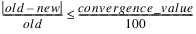
When old or new is zero, convergence is reached as follows:
if 
Example | Convergence? | Explanation |
|---|---|---|
old = 100.0 cms new = 100.001 cms convergence value entered = 0.001 | Yes | |
old = 10.0 cfs new = 10.01 cfs convergence value entered = 0.001 | No |  |
Unit Percent
Absolute difference, in user-specified units. The user enters the convergence value as a percentage, without regard to scale.
Convergence is reached as follows:
if 
Example | Convergence? | Explanation |
|---|---|---|
old = 100.0 cfs new = 100.001 cfs convergence value entered = 0.1% cfs | Yes | |
old = 10.0 cfs new = 10.1 cfs convergence value entered = 0.1% cfs | No |  |
Time Series Range—Series Slot
The default start times and timestep are inherited from the Run Control settings when the object is instantiated. All series slots are initialized with one timestep to minimize model file size. Other rows are added by the user as needed for input or appended at run time when the slot’s output values are calculated. You may change the time series range directly through the Time Series Range Dialog.
On Integer Indexed Series, the user is able to change the number of Values but the start, end, and timestep size configuration areas are disabled.
The time series range and timesteps can also be changed by selecting Sync With Run Control in the Time Series Range Dialog. This will update the time series range in the slot to match the time series range set in the Run Control dialog. The default start times and timestep are inherited from the Run Control settings when the object is instantiated.
Linked Slots
In the View menu, there is a menu to show Linked Slots. When selected, this shows all of the slots to which the given slot is linked.
Show Notes Column and Notes Group Menu
The Show Notes Column and the Notes Group menu are used to display Notes that are associated with a timestep on a series slot. See Notes on Series Slots for details.
Series Display Compression
The Series Display Compression utility allows the user to compress or hide a particular value, NaNs, both, or any repeated values. This utility is useful for slots that hold data that is often the same value and the user only wishes to see any changes to this standard value. The functionality is available on Series Slots, Agg Series Slots, Multi Slots, and Table Series Slots.
Accessing Series Display Compression
Series Display compression can be accessed from
• Open Slot dialog View, then Series Display Compression menu.
• Series Display Compression icon  on the Open Slot dialog.
on the Open Slot dialog. When either of these options are chosen, the Open Slot dialog adds the display compression area between the scroll area and above the column heading.
Configuring Compression
Figure 5.16 identifies the configuration controls. Each control is described in detail.
Figure 5.16
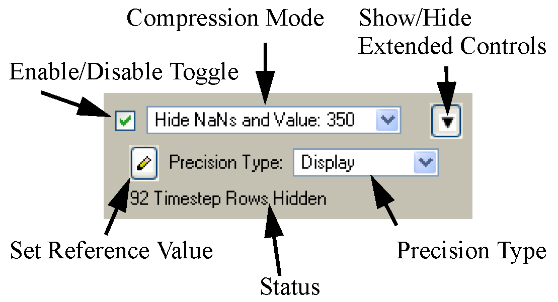
Enable/Disable Toggle
When Series Display Compression is first activated, there is a check mark in the toggle indicating that it is active. This toggle is used to toggle the compression on and off. Thus, the user can configure compression, then toggle it off to view or edit all the values, and then toggle it back on to reenable compression
Compression Mode menu
When first activated, the Compress Repeated Values option is selected by default in the Compression Mode menu. The following modes are available for display compression:
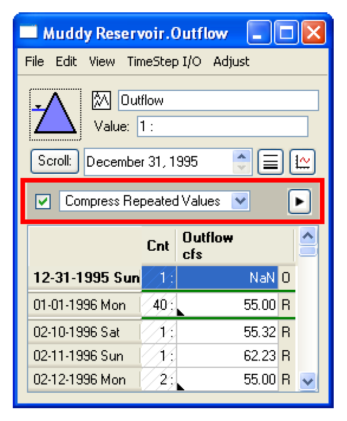
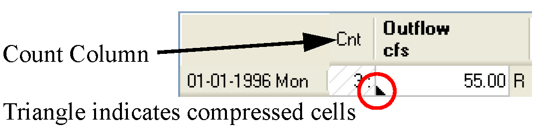
• Compress Repeated Values. Any values that are repeated will be compressed into one row. When this option is selected, the repeated values are all compressed into one cell and a count (Cnt) column is added. A small triangle is added to the lower corner of the cell to indicate that the cell represents repeated values. In the screenshot 3 values of 55cfs are repeated on 1/1/1996. These represent 1/1 through 1/3/1996.
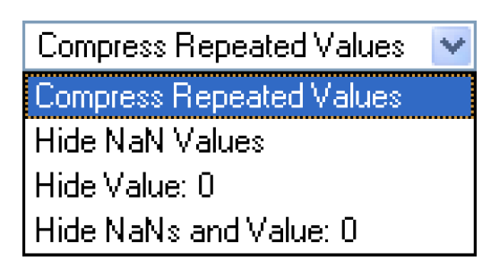
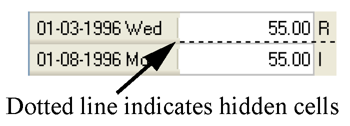
• Hide NaN Values. All NaN values will be hidden and a dotted line is shown. For example, NaNs are hidden for 1/4 through 1/7/1996.
• Hide Value: #. All values matching the reference value will be hidden and a dotted line is shown. The user can change the value by selecting the Reference Value icon  and entering a new value.
and entering a new value.• Hide NaNs and Value: #. All NaN values or values matching the reference value will be hidden and a dotted line will be shown. The user can change the reference value by selecting the Reference Value icon  and entering a new value.
and entering a new value.• Show Value: #. All values that match the reference value are shown. NaNs are hidden. The user can change the reference value by selecting the Reference Value icon  and entering a new value.
and entering a new value.• Show NaNs and Value: #. All NaNs and values that match the reference value are shown. The user can change the reference value by selecting the Reference Value icon  and entering a new value.
and entering a new value.• Show Values <= #. All values less than or equal to the reference value are shown. NaNs are hidden. The user can change the reference value by selecting the Reference Value icon  and entering a new value
and entering a new value• Show Values >= #:All values greater than or equal to the reference value are shown. NaNs are hidden. The user can change the reference value by selecting the Reference Value icon  and entering a new value
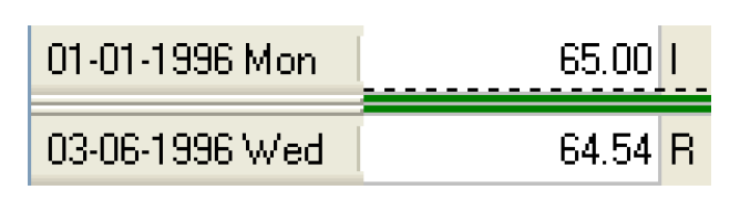
and entering a new valueNote: The above text describes the options and how RiverWare represents each option on the screen. In each case, if the compressed/hidden range contains the automatic green DateTime interval delineations (e.g. Monthly lines on a slot with a 1 Day timestep) those green lines will still be shown. In the example to the right, two green lines are shown representing the delineation before Feb. 1 and March 1 in this 1 Day timestep slot.
Show/Hide Extended Controls
To the right of the Compression Mode menu, the Show/Hide Extended Controls button  can be used to further refine how the compression is configured. When this button is selected, additional configuration options are presented, and the arrow points down.
can be used to further refine how the compression is configured. When this button is selected, additional configuration options are presented, and the arrow points down.Set Reference Value
When any of the Hide Value or Show Value compression modes are selected, the Set Reference Value icon  become active. Selecting this icon opens a dialog to allow the user to enter a value. Once a new number is entered, the Compression Mode menu options will display that number in the menu. The value does not have a unit associated with it. So if you change the slot’s units (via the configuration or through a unit scheme), the reference value will not change.
become active. Selecting this icon opens a dialog to allow the user to enter a value. Once a new number is entered, the Compression Mode menu options will display that number in the menu. The value does not have a unit associated with it. So if you change the slot’s units (via the configuration or through a unit scheme), the reference value will not change. Precision Type menu
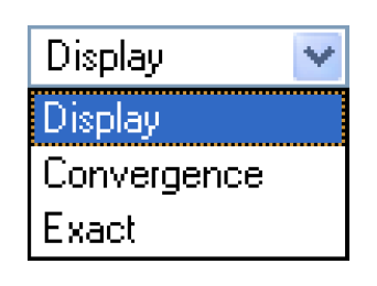
Each of the above compression modes compares a value in a cell to some other value, either a reference value, NaN or the previous timestep’s value. For more flexibility, value comparison can be based on either:
• Display. The display precision will be used; this is the default. If two numbers appear the same on the screen, they are considered the same.
• Convergence. The slot’s convergence value will be used to compare the numbers. A number must be within convergence of the other number to be considered the same.
• Exact. The internally stored numbers will be compared.
Status information
The Status information will show the number of rows that are hidden or compressed.
Editing Compress and Hidden Values
On the Open Slot dialogs, the user can highlight a number of cells and type a new value that will be entered, as Input, into each selected cells. When Series Display Compression is enabled, the editing of values is treated a differently as follows:
Compressed Repeated Values
If the Compress Repeated Values is selected, editing of selected cells will edit any compressed cells. For example, if repeated 33 values are repeated and the user selects the repeated value, types in a new number, all 33 values will be set to that new number.
Hidden NaNs or Value
If any of the Hide options are selected, editing of selected cells will not affect hidden cells. Hidden values and NaNs will not be overwritten. But, any cells displayed and selected will be affected by the new value. Also, if the entire column is selected, edits will then apply to all values, whether hidden or not.
Multi-column Slots
On multi-column slots, (Agg Series, Multi Slots, Table Series Slots, and accounting slots), the Series Display Compression will only compress/hide a row if the compression is valid on all columns of the row. In Figure 5.17, repeated value compression only applies to a subset of rows.
Figure 5.17
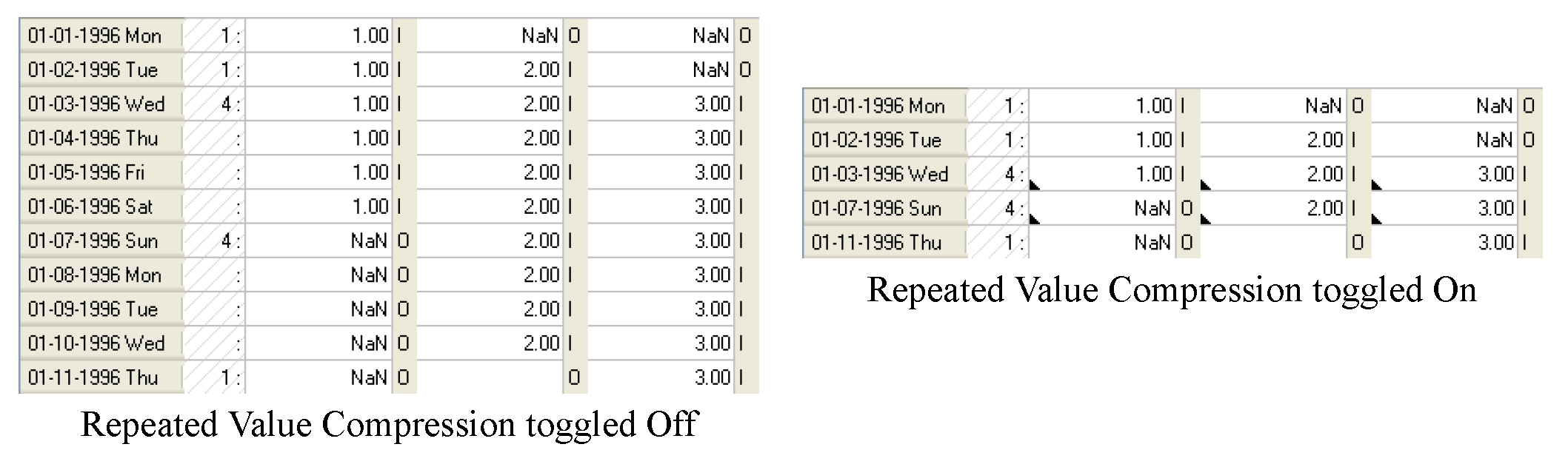
Note: Only rows 1/3–1/6 and 1/7–1/10 are compressed because the repetition occurs across all columns. Similarly, on multi-column slots, if the user selects the Hide NaNs and Value option, it will only hide a row if all three columns have the reference value OR NaN.
Flags on the Timestep I/O Menu
On Series Slots, the Timestep I/O menu is used to change the status of the cell’s value by changing the flag. Possible flags vary by slot, but may include the following:
• INPUT (I)
• OUTPUT (O)
• DMI INPUT (Z)
• ITERATIVE MRM (i)
• TARGET BEGIN (TB or tb)
• TARGET (T)
• BEST EFFICIENCY (B)
• MAX CAPACITY (M)
• DRIFT (D)
• SURCHARGE RELEASE (S)
• REGULATION DISCHARGE (G)
• UNIT VALUES(U)
• RULE (R)
User-input data are automatically flagged as INPUT, and may not be overwritten by simulation results. Certain values imported by an input DMI are flagged Z for DMI INPUT and are treated identically to INPUT (I) flags. Initialization Rules can also set values with the Z flag. OUTPUT (O) timesteps may contain values calculated during a previous run or toggled from INPUT status. These values are automatically cleared to NaN at the beginning of a simulation run. This guarantees that no previous solutions remain from one run to the next. Simulation results are written to timesteps flagged as OUTPUT, TARGET BEGIN, BEST EFFICIENCY, MAX CAPACITY, SURCHARGE RELEASE, DRIFT and UNIT VALUES. Flags other than OUTPUT and INPUT are only available for certain series slots.
Special Series Slot Flags
This section describes the use of special flags which may be set on Series Slot timesteps. The flags are typically set by the same mechanisms as INPUT and OUTPUT flags. But, unlike INPUT and OUTPUT flags, each type of special flag is only applicable to one or two slots. All SeriesSlots must have one of the following flags set for every timestep; each flag is indicated by its abbreviation:
• General flags available to all SeriesSlots.
– I for INPUT
– O for OUTPUT
– Z for DMI INPUT. This flag indicates that the value was set by an input DMI or Initialization Rule. See DMI Invocation Manager Dialog in Data Management Interface (DMI) for details on DMI Invocations. See Initialization Rules Set in RiverWare Policy Language (RPL) for details on Initialization Rules. In simulation, the Z flag behaves identically to the INPUT (I) flag.
– R for SET BY RULE. This flag indicates that the value was set directly by a rule.
– i for ITERATIVE MRM. This flag indicates that the value was set during iterative MRM by an MRM rule. Values with the “i” flag can be overwritten as though it is a “O” flag. Values with the “i” flag are cleared at the beginning of a single run and at the start of an MRM run, but are not cleared between each iterative MRM run. They are considered input during an iterative MRM run.
• Power calculation flags available to Energy slots.
– B for BEST EFFICIENCY
– M for MAX CAPACITY
• Maximum Outflow flag available to Outflow slots
– M for MAX CAPACITY
• Target flags available to Storage and Pool Elevation slots.
– TB or tb for TARGET BEGIN
– T for TARGET
• Drift flag available to Regulated Spill and Bypass slots.
– D for DRIFT
• Surcharge Release flag available to the Surcharge Release slot
– S for SURCHARGE RELEASE
• Regulation Discharge flag available to the Regulation Discharge slot
– G for REGULATION DISCHARGE
• Unit Values flag available to Turbine Release and Energy slots on power reservoirs with the Unit Power Table method selected:
– U for UNIT VALUES
Setting Flags
Flags are set from the Open Slot dialog or from the SCT. In the Open Slot dialog, a flag is set on the highlighted timestep by selecting the flag from the Timestep I/O menu. Flags which are unavailable for that slot will appear dimmed in the menu.
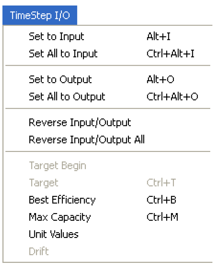
The Timestep I/O menu has the following options:
• Set to Input. Set selected cells to Input
• Set All to Input. Set all cells to Input
• Set to Output. Set selected cells to Output
• Set All to Output. Set all cells to Output
• Reverse Input/Output. Reverse the input and output flags on selected cells
• Reverse Input/Output All. Reverse the input and output flags on all the cells
• Set one of the special flags on the selected cells. The following sections describe many of the special flags.
Power Calculation Flags on Energy
BEST EFFICIENCY and MAX CAPACITY flags may be set on Energy timesteps instead of an INPUT Energy request value. These flags are used by the Plant Power Coefficient Release User Method to calculate the most efficient or maximum Energy generation possible for the flagged timestep.
The Plant Power Coefficient Release method uses tables to relate the current Operating Head to the most efficient Turbine Release or maximum allowable Turbine Release. The MAX CAPACITY flag is available for all power method except LCR Power Calc. The BEST EFFICIENCY flag is only valid for the following power methods:
• Plant Power Coefficient
• Plant Efficiency Curve
• Plant Power Equation
• LCR Power Calc
• Unit Power Table
The calculation of the best efficiency Energy generation or max possible Energy generation is an iterative solution. The Outflow required to produce the desired type of Energy affects Tailwater Elevation, which affects Operating Head, which affects the Outflow required to produce the desired Energy. See Power Release in Objects and Methods for details on this methods.
When an energy value has been calculated using a MAX CAPACITY or BEST EFFICIENCY flag and it is set as a user input for a subsequent run, a warning may be posted that says “Energy request cannot be met on current iteration.” This is due to the way RiverWare solves. When two reservoirs are modeled in series, the Tailwater Elevation of the lower reservoir affects the Operating Head of the upper reservoir. The Outflow of the upper reservoir, in turn, affects the Tailwater Elevation of the lower reservoir. This creates an iterative loop between the Outflow from the upper reservoir, the Tailwater Elevation of the lower reservoir, and the Operating Head of the upper reservoir. When an Energy value is set using either a MAX CAPACITY or a BEST EFFICIENCY flag, the reservoirs iterate over Outflow, Tailwater Elevation, and Operating Head until the values converge. If the Energy value is now set as an input and the model is run again, the Input Energy may not be possible given the Operating Head on the first iteration. If this happens a RiverWare warning is posted but the run does not abort, since the energy value MAY match the Operating Head at a later iteration. The Energy also MAY NOT match the Operating Head at a later iteration. If this occurs, the model will continue running even though the object did not solve. The run will NOT be aborted, but objects may not dispatch because required information was not propagated to them. The user must check the dispatch dialog if they receive the RiverWare warning message given above to make sure the model ran correctly.
Maximum Capacity Flag on Outflow
As demonstrated in the simulation exercise, this flag computes the maximum possible Outflow from a Reservoir on a given timestep. Setting the MAX CAPACITY flag on a Reservoir Outflow slot forces the Outflow to equal the sum of the maximum (Turbine) Release and the maximum Spill.
Caution: Take care when using this flag, as its effects may cause downstream reservoirs to exceed their operating ranges. The use of this flag also depends on having reliable and accurate input tables relating elevation to maximum release and spill.
The MAX CAPACITY flag is set by highlighting a simulation timestep on the Outflow slot of a Reservoir and selecting Timestep I/O, then Max Capacity. RiverWare places an M at the selected timestep to indicate that the flag is active. This flag is treated as an INPUT, but does not require a value. If a valid Outflow value is present at the flagged timestep, it is ignored in the simulation; a new Outflow value is calculated and displayed at that timestep. This behavior is similar to the Max Capacity and Best Efficiency flags of the Energy slot and the Drift flags of the Regulated Spill and Bypass slots. A Reservoir which has the Outflow Max Capacity flag set may dispatch under any of the “given Outflow” dispatch methods, as follows:
• Solve given Outflow, Pool Elevation for Level Power, Slope Power, and Storage Reservoirs.
• Solve given Outflow, Storage for Level Power, Slope Power, and Storage Reservoirs.
• Solve given Inflow, Outflow for Level Power, Slope Power, Pumped Storage and Storage Reservoirs.
The Outflow Max Capacity flag may NOT be used on reservoirs when solving for Hydrologic Inflow, or when solving a Target Operation.
The Max Capacity solution is iterative. The exact sequence of calculations in each iterative loop is dependent on the type of Reservoir and the selected Spill Calculation Method. In all cases, the maximum Spill and maximum controlled Release are calculated individually, then summed. If the selected Spill Method includes Regulated Spill, the current or previous Pool Elevation is used to look up the maximum Regulated Spill from the Regulated Spill Table. This value is set in the Regulated Spill slot, and the selected Spill Calculation Method is called. Any input Bypass and/or required Unregulated Spill are considered within the Spill Method. Next, the maximum release is calculated. If the Reservoir is a Power Reservoir, the selected Tailwater method is executed to determine the Operating Head. This Operating Head or the Pool Elevation (in the case of Storage Reservoirs) is used to look up the maximum release from the Max Turbine Q table, Max Release table, Max Flow Through Turbines table, or Best Generator Flow table. Finally, the maximum release and the calculated Spill are added to determine the total maximum Outflow. This Outflow is used to mass balance the Reservoir. The iteration is repeated until Convergence is met or Max Iterations is exceeded.
Target Operation Flags
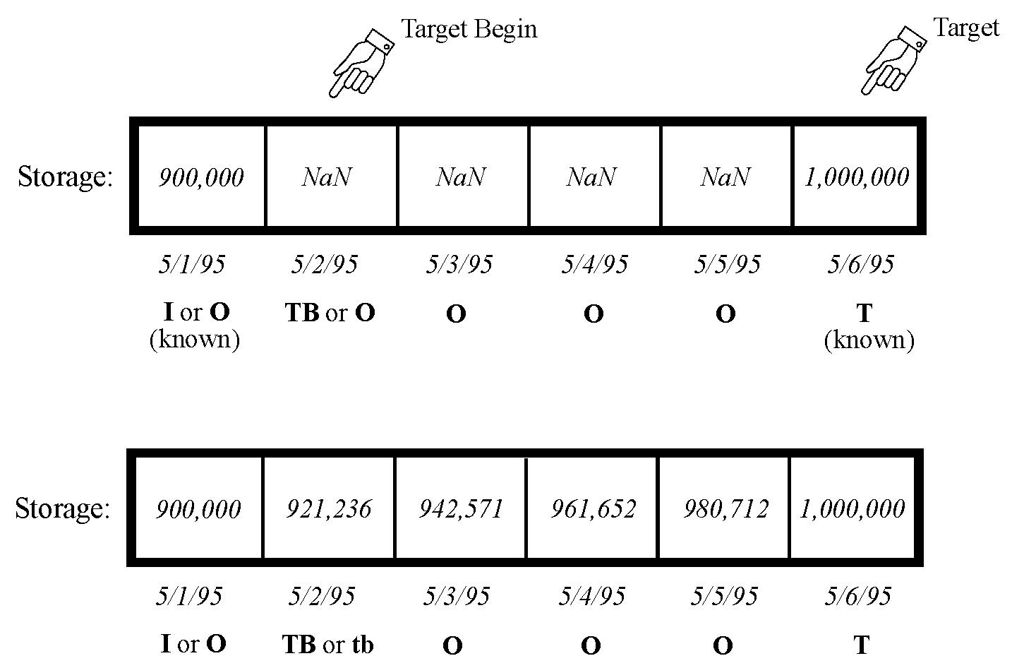
Target Operations are used to calculate a lumped mass balance across several timesteps, in order to exactly meet a user-input TARGET Pool Elevation or Storage value. Three conditions are necessary for a Target Operation to execute successfully:
• An initial value must be known at the timestep before the TARGET BEGIN timestep. This value may be INPUT or a known value at the time the Target Operation solves.
• A target Pool Elevation or Storage value must be specified at the TARGET timestep.
• Either Inflow or Outflow must be known for all timesteps in the target range.
Given these conditions, RiverWare calculates the unknown Inflows or Outflows for all of the timesteps within the Target Operation, such that the TARGET value is exactly met.
Timestep Range
When solving a target operation, RiverWare searches backwards from the TARGET time until it finds a valid TARGET BEGIN flag. The Target Operation is solved using the value from the timestep prior to the TARGET BEGIN flag as an initial condition. If the timestep prior to the TARGET BEGIN does not have a valid Storage or Pool Elevation, or a valid input value exists between the TARGET BEGIN and the TARGET, the simulation aborts with an error. Likewise, if the TARGET BEGIN or TARGET timestep already has enough information to dispatch with a different dispatch method, simulation aborts. If no TARGET BEGIN flag is specified, RiverWare searches backwards to the first valid value and solves the Target Operation with this initial condition.
When a beginning of target is assumed in this manner, RiverWare marks the timestep where the Target Operation actually begins with a tb (lowercase) flag in the Open Slot dialog. This flag is treated as an output, and is automatically cleared at the start of the next run. Setting a Target Operation from an SCT generates both the TARGET and TARGET BEGIN flags, and clears any previous Target Operations which overlapped with the new range.
Lumped Mass Balance
To calculate the unknown flow values, RiverWare performs a lumped mass balance over the target range. The required change in Storage is found by subtracting the storage just before the TARGET BEGIN (converted from Pool Elevation in the case of a Pool Elevation TARGET) from the TARGET value (also converted from Pool Elevation in the case of a Pool Elevation TARGET). All of the known Inflows and/or Outflows are then summed to calculate a side flow gain or loss of Storage over the target range. This volume of side flows is then subtracted from the change in Storage required to meet the TARGET value, and the remaining flow volume is distributed equally among the unknown Inflows or Outflows. Equation 5.1 and Equation 5.2 represent these calculations.
(5.1) 
(5.2) 
Redispatching
The setting of flow values on intermediate timesteps of the Target Operation forces the object onto the dispatch queue at those times. The timesteps dispatch with enough information to solve completely (Inflow and Outflow are known for all timesteps.) The only timestep which actually re-dispatches is the TARGET timestep, since a valid previous Storage value is now known.
Spill Drift Flags
Spill DRIFT is used to calculate the Regulated or Bypass Spill over a controlled gate as the reservoir Pool Elevation changes over time. The flag is always considered an input on any timestep where it is set but no value is initially set by the user. In this way, it is similar to the Energy BEST EFFICIENCY and MAX CAPACITY flags. Since DRIFT is considered an INPUT, it may affect over determination of Spill parameters.
The first timestep prior to initiating drift is used to determine a gate index called the Regulated (or Bypass) Drift Index. This index is interpolated from a 3-dimensional Regulated (or Bypass) Spill Index Table, which relates Pool Elevation to Spill for various gate indices. In all subsequent timesteps where the DRIFT flag is set, the same index is used to determine the new Spill. The gate index is maintained throughout the selected time period. At each timestep, the new value of Spill is calculated for the structure based on the current average Pool Elevation.
Surcharge Release Flag
The SURCHARGE RELEASE flag is used to calculate the surcharge or mandatory release from a reservoir during flood control operations. Surcharge releases are meant to evacuate water from that sits above the top of the flood pool. This flag can only be set on the Surcharge Release slot which is only available when the user has selected a Surcharge Release method. The flag is always considered an input on any timestep where it is set but no value is initially set by the user.
Although the SURCHARGE RELEASE flag may be set by selecting Timestep I/O, then Surcharge Release from the Surcharge Release slot, in practice it should only be set by a rule. When the SURCHARGE RELEASE flag is set, and the inflow to the reservoir is known, the reservoir can dispatch with the Solve given Inflow, Outflow dispatch method. This dispatch method will calculate the forecasted surcharge releases and will set them on both the Surcharge Release and Outflow slots so that they may propagate downstream. The manner in which the forecasted surcharge releases are calculated depends on the method selected in the Surcharge Release category. If you are interested in using one of the surcharge release methods, see Surcharge Release in Objects and Methods for details.
Regulation Discharge Flag
The REGULATION DISCHARGE flag is used to calculate the regulation discharge at a Control Point. Regulation discharge is used during flood control operations and is defined as the maximum allowable flow in the channel at the control point. This flag should only be set on the Regulation Discharge Calc slot on Control Points. This slot is only available when the user has selected a Flood Control method and a Regulation Discharge method. The flag is always considered an input on any timestep where it is set but no value is initially set by the user. Like the SURCHARGE RELEASE flag, the REGULATION DISCHARGE flag should only be set by a rule. If you are interested in using one of the Regulation Discharge methods, see Regulation Discharge in Objects and Methods for details.
Unit Values Flag
The UNIT VALUES (U) flag is used to indicate that the user is going to specify unit level values but would like to use those to drive the solution. The UNIT VALUES flag may be set on Energy or Turbine Release on power reservoirs that have the Unit Power Table method selected (see Unit Power Table in Objects and Methods). If the Unit Power Table method is not selected, an error is issued. This flag is considered a user input but does not require a value (similar to the MAX CAPACITY and BEST EFFICIENCY flag). At the beginning of the run any numeric values are cleared out. The flag can be set directly on the slot, from the SCT, or from a Rule.
U Flag on Energy
Thus, if the U flag is set on Energy, one or more Unit Energy subslots must be specified by user input or a rule. When RiverWare runs, it sees that Energy has this flag which is considered an input. If it has enough other information (like Inflow, Storage, or Pool Elevation), the reservoir will be able to dispatch one of the following methods:
• Solve given Energy, Inflow
• Solve given Energy, Storage
• Solve given Energy, Pool Elevation
In addition, Energy can be flagged U, if the reservoir dispatches one of the following methods:
• Solve given Inflow, Outflow
• Solve given Outflow, Pool Elevation
• Solve given Outflow, Storage
These methods do not require Energy to be unknown.
U Flag on Turbine Release
Alternatively, if the U flag is set on Turbine Release, one or more Unit Turbine Release subslots must be specified as user input or by a rule. When RiverWare runs, it sees that Turbine Release has this flag which is considered an input. If it has an Inflow, the reservoir will be able to dispatch the Solve given Inflow Release method.
This flag is specific to the Unit Power Table method; see Unit Power Table in Objects and Methods for full details on this algorithm.
Finding Inputs
The Find Series Slots with Inputs utility can be used to find values that are input in the model. It is accessed from the RiverWare Workspace using the Workspace, then Slots, then Find Inputs menu. The Search Slots dialog appears.
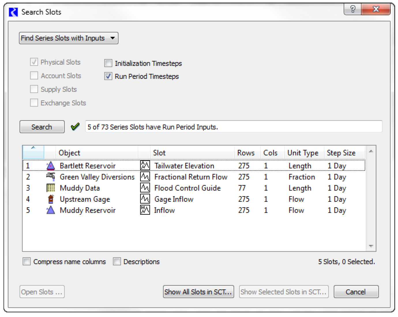
The user has options to filter on the types of series slots on which to look for input values. In a pure simulation model, this is only Physical Slots (i.e. Outflow, Inflow, etc.) If Accounting is enabled, the user may choose to search any or all of the following series slot “domains”:
• Physical Slots
• Account Slots
• Supply Slots
• Exchange Slots
The search may be limited to either Initialization Timesteps (before the Run Start timestep) or Run Period Timesteps (on or after the Run Start timestep). If both are checked, all series slots having any inputs are found, regardless of where (in time) those Input values are within the slots' time series.
The search operation is performed by selecting the Search button. The number of series slots with Input-flagged timesteps, and the total number of series slots matching the checked “domains” are indicated in a status line to the right of the search button. If search criteria is changed (by selecting any of the checkboxes at the top of the dialog), a green check icon  is displayed next to the search button indicating that a new search with the new criteria has yet to be performed. The green check icon is hidden upon performing another search.
is displayed next to the search button indicating that a new search with the new criteria has yet to be performed. The green check icon is hidden upon performing another search.The user has the option of showing the slots' object name and account name (if applicable) in separate columns. This is controlled by the Compress columns checkbox below the slot list. This is not available if supply slots or exchange slots are shown in the slot list,
Several context menu (right-click) operations are available within the slot list:
• Open Slot. Show the open slot dialog for the picked slot item.
• Open Object. Show the object dialog for the picked slot item (if applicable).
• Copy Slots. Put the selected slot items into the slot clipboard, e.g. to paste into an output (manager) device slot list.
Buttons along the bottom of the dialog provide these functions:
• Open Slots. Separate open slot dialogs are shown for each of the selected items in the list. If more than four (4) slots are selected, then a query dialog box is shown confirming the operation with a message like this: “Do you want to show 421 Open Slot dialogs?”.
Note: All shown open slot dialogs may be hidden with the Workspace, then Slots, then Close All Slots menu operation.
• Show All Slots in SCT. All slots in the list (regardless of item selection) are shown in a new SCT dialog, and the Find Series Slots with Inputs dialog is closed.
• Show Selected Slots in SCT. Selected slots in the slot list are shown in a new SCT dialog, and the Find Series Slots with Inputs dialog is closed.
• Cancel. The Find Series Slots with Inputs dialog is closed.
The dialog can also be used to find slot descriptions; see Slot Descriptions for details.
Series Slots With Expression
Expression slots are computational expressions. The user can either create a Series Slot with Expression or a Scalar Slot with Expression. They are used to calculate quantities such as “combined Storage of all Reservoirs,” “weekly average Outflow of Hoover Dam,” “the ratio of Hydrologic Inflow to Reach Inflow at selected structures”, or any conceivable expression. To add a Series slot with expression select Slot, then Add Series Slot with Expression.
Expression slots utilize the RiverWare Policy Language (RPL). RPL is computationally expressive language and has an associated structured editor. Because Expression slots utilize RPL (the same language in which RiverWare rules are written) they may contain simple expressions or complex logic and functions. Anything that may be expressed in a rule may also be evaluated in an Expression slot. The use of RPL also provides dimensional analysis to ensure that units are reconciled throughout the expression.
Note: Ensure that the unit type of the slot is the same as the units to which the expression evaluate.
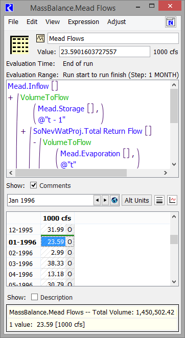
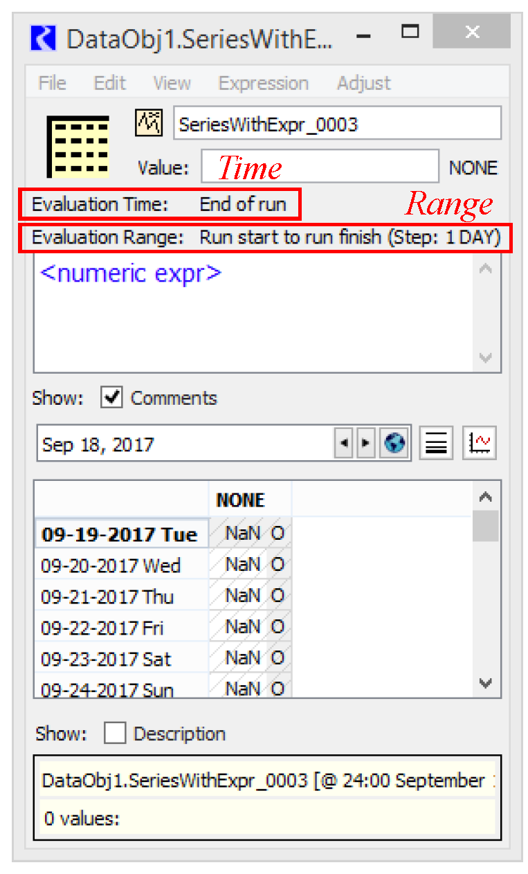
When first opened, this slot is shown in its own Slot Dialog so you can see and edit the expression or the data. A sample is shown in Figure 5.18.
Figure 5.18 Screenshot of a Series Slot with Expression
The slot can also be shown in the Slot Viewer, with only the data shown. Use the File menu or drag the slot onto the viewer as described Slot Viewer Functionality. When this type of slot is shown in the Slot Viewer, there is special ornamentation in the column heading indicating its type, as shown in Figure 5.19, indicating there is an expression to edit or view. Click the icon  to open the slot in its own dialog where you can see the expression.
to open the slot in its own dialog where you can see the expression. Figure 5.19 Screenshot of the Series Slot with Expression shown in the Slot Viewer.
Configuration
Following is description of the configuration options available for expression slots. All of these menus can be accessed from the Slot Dialog. All but the Expression menu can be accessed from the Slot Viewer.
File Menu
On the File menu, the Import options are not available as you cannot import or type data into the slot. The export options are available and can be used to export the calculated data out of the slot. A Print Expression menu option is available to print the expression. This uses the same printing mechanism as other RPL sets; see Printing in RiverWare Policy Language (RPL) for details.
Edit Menu
On expression slots, the Edit menu has options to Copy (to the RiverWare clipboard) and Export Copy (to the system clipboard). Importing, pasting, and other data editing features are disabled as the expression slot is “output only”.
View Menu
The View Menu on expression slots show the following menu options.
Configure
The configuration uses the standard series slot configuration dialog; see Configure Slot Dialog Functionality for details. You can change the unit type of the expression slot. It must correspond to the unit type of the RPL expression.
Evaluation Range
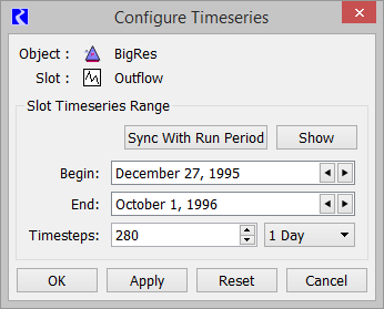
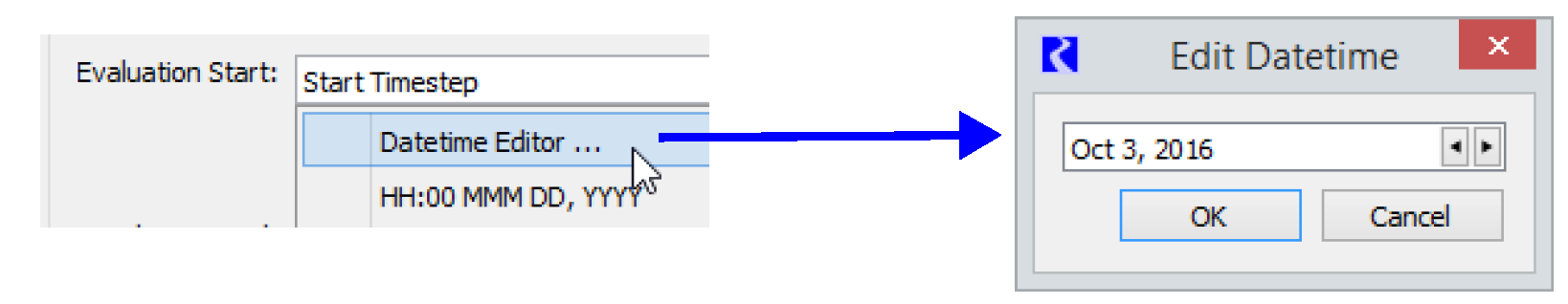
By default, Expression slots are evaluated for each timestep in the model run (i.e., the range is synchronized with the run control). If you are only interested in the result of an expression for a reduced range of dates or for a different timestep, you may select View, then Evaluation Range, to open the Configure Timeseries—Evaluation Range dialog and enter the date range in which you are interested.
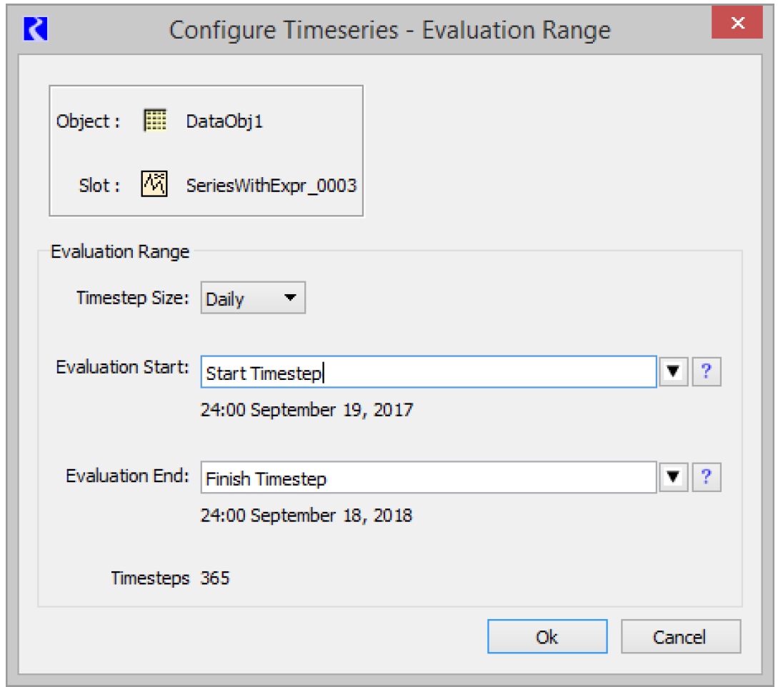
The Start and End times can be specified explicitly or symbolically as RPL DATETIMES; see DATETIME in RiverWare Policy Language (RPL) for details. Text below the editor field indicates the actual DateTime of the entered symbolic time text (if it is valid), or the status if it is not valid. You can also use the menu to specify one of the common DateTimes. Some of these are expressions that must be edited to become valid, e.g. by replacing “N” with a nonnegative integer and the HH:00 MMM DD, YYYY formula, where you substitute the hour, month, day and year.
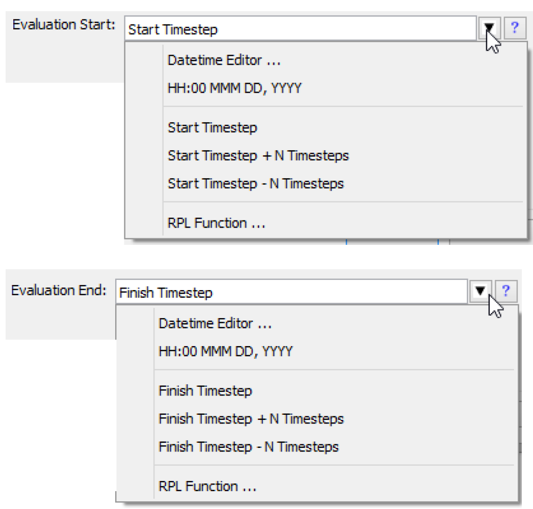
The Datetime Editor option opens a separate dialog to specify the DateTime using a selector configured for the model's timestep size.
The RPL Function opens a Function Selector to select a RPL function in the Expression Slot or Global Function Set. The selected function must have a return type of DATETIME, and must not have any arguments.
Select Help (question mark icon button) on the right side of the symbolic DateTime editor to show a description of symbolic DateTime representations.
Note: An expression slot does not need to have the same timestep as the run control. For slots with a different timestep than the run, the slot will evaluate for only those timesteps that fall within the run dates. When entering a symbolic date such as “Start Timestep—N Timesteps”, the slot's timestep will be used in the subtraction.
Expression Menu
Show Expression
This toggle is used to show or hide the expression. By default, the expression is shown.
Evaluate
The user can manually evaluate the expression from the Expression, then Evaluate menu.
Validate
The user can manually verify the expressions validity using the Expression, then Validate menu.
Evaluation Time
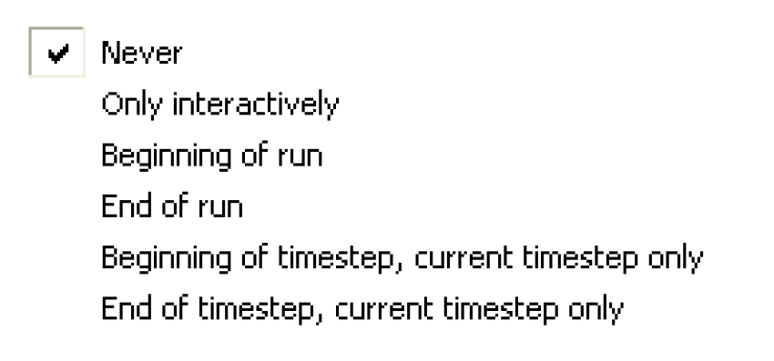
Expression slots can be evaluated at the beginning or end of each simulation run, at the beginning or end of each timestep, never, or interactively on demand. These options are particularly useful for performance when running large models and when evaluating a large number of expression slots. To select when an Expression slot is evaluated select Expression, then Evaluation Time from the Expression slot menu and select an option. A check mark will be shown next to the selected option.
Note: Unlike rules, expression slots do not reevaluate if dependent slots change, but if the expression slot returns a NaN, the expression slot is put on a list of slots to be re-evaluated during that same evaluation time. The NaN might come from an expression slot that hasn't been evaluated yet, so it should evaluate later, once that expression has had a chance to evaluate. The palette operations IsNaN and NanToZero return a valid value, so do not cause re-evaluation of the expression slot.
Editing Menu items
The Expression menu is used to build expressions. There are options to Cut, Copy, Paste, Delete, and Enable and expression. Undo and Redo are available to go back or go forward when editing expressions. These are only available when a relevant expression is selected. Finally, there is a menu option to bring up the Palette open the RPL Debugger and open the RPL set.
Open RPL Set
The RPL set containing functions used by any expression slot can be opened by View, then Open RPL Set. All of the functionality associated with a RPL set can be utilized from this RPL set editor such as importing/exporting, analysis, search and replace, and creating utility groups of functions.
Note: Only functions are shown in the RPL set editor; the expressions on the slots themselves are the equivalent to the rules in a ruleset. See About RPL Sets in RiverWare Policy Language (RPL) for details on RPL sets. From the RPL set, the user can control the layout using the Set p Layout menu. See Formatting: Display Settings in RiverWare Policy Language (RPL) for details on layouts.
Show Comments
The Show Comments menu allows you to hide or show inline RPL comments (added from the palette). There is also a toggle on the slot dialog below the RPL expression that hides/shows the comments. Comments are shown by default. If there are any comments defined, a box is shown around the toggle.

Building Expressions
Expression slots utilize the RPL palette to build expressions. The RPL palette provides a syntax-guided editor designed to assist in the construction of complex syntactically correct expressions within the RiverWare Policy Language environment. The editor works by maintaining a partially constructed expression and allowing the user to manipulate unfinished portions using the palette. Initially, the buttons in the palette are grayed out. When building an expression, the palette enables any buttons that could possibly go in a highlighted portion of the expression.
See Editing a RPL Expression in RiverWare Policy Language (RPL) for details.
Note: For Expression Series Slots, the symbolic DateTime specifications @”Start Timestep” and @”Finish Timestep” refer to the expression slot’s evaluation range, not the controller’s start or end dates. The predefined functions RunStartDate() and RunEndDate() provide a reference to the controller’s start and end dates, respectively. See RunStartDate, RunEndDate in RiverWare Policy Language (RPL) for details.
Tip: For Expression Slots, you can use the keyword ThisObject to access the containing object. For example, to get the slot named DailyTotals from this object, you could create the following expression:
ThisObject. “DailyTotals”[]
Diagnostics for Expression Slots
Diagnostics for expression slot evaluation can be configured in the Diagnostics Manager; see Diagnostics Manager in Debugging and Analysis for details.
If expression slots are evaluated outside of a run, using the Expression, then Evaluate menu on the slot or the Control, then Evaluate Expression Slots menu from the workspace, then diagnostics must be set up using the Workspace diagnostics; see This document is under development. in Debugging and Analysis.
If expression slots are evaluate during a run, either beginning or end of timestep or beginning or end of run, then diagnostics must be set up using Simulation diagnostics (see Simulation Diagnostics in Debugging and Analysis) or Rulebased Simulation diagnostics (see Rulebased Simulation Diagnostic Groups in Debugging and Analysis), depending on the selected controller. Within each of those diagnostics configurations, the Expr. Slot Execution and Expr. Slot Function Execution categories deal with expression slots.
Text Series Slots
The Text Series Slot holds a series of user-specified text strings. Because it is a series slot, it provides much of the required series slot functionality like display, flags, use in SCTs, and input via DMI. Figure 5.20 shows a sample Text Series Slot. It has comments about how the system is operated during Flood Season.
Figure 5.20 Screenshot of a Text Series Slot
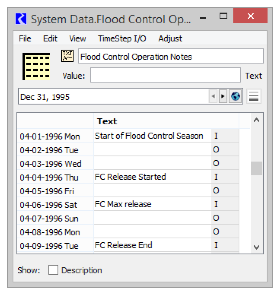
Note: Internally, the Text Series Slots is a normal series slot that holds an encoded index which indicates which text string to display. If you try to copy and paste, you will see the encoded number.
The following list provides information on supported functionality:
• The Text Series Slots behaves like other slots in terms of showing/hiding/grouping on the open object dialog. They have a description and other normal slot attributes.
• Text values have normal, I, O, and Z flags. A non-specified value is blank, not NaN.
• Convergence, bounds, and changing units on Text Series Slots is not relevant.
• Import/Export through a DMI is supported via Excel Database DMIs; see Excel Datasets in Data Management Interface (DMI) for details.
• Text Series Slot values can be displayed and edited in an SCT.
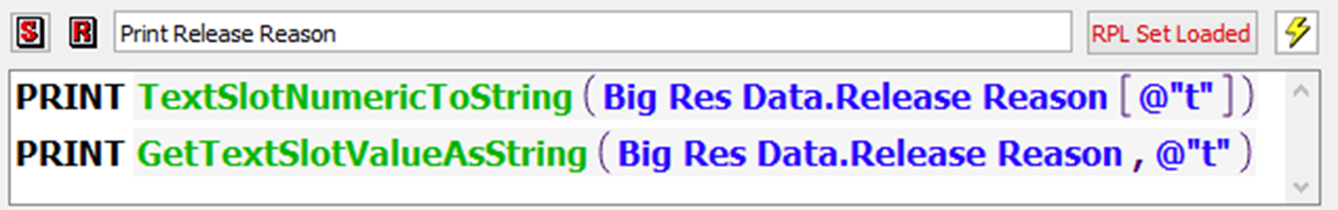
• Text Series Slot values can be read by RPL using the following RPL predefined functions. Samples are shown in Figure 5.21.
Figure 5.21 Image of RPL functions accessing a Text Series Slot.
• Text Series Slot values can be set by rulebased simulation rules or initialization rules using the function StringToTextSlotNumeric in RiverWare Policy Language (RPL). This function converts a string to a value that can be stored in the slot. The assignment syntax, as shown in Figure 5.22, is as follows:
Object.TextSeresSlot[ ] = StringToTextSlotNumeric(“Text string to set”)
Figure 5.22 Image of rule assignment setting a Text Series Slot

As of version 7.4, the following functionality is not supported:
• Import/Export to a text file is not allowed.
• Text Series Slot are not displayable in Model Reports of Tabular Series Slot Reports
• Text Series Slots can not be set by script actions.
• Text Series Slots can not be set by iterative MRM rules or Object Level Accounting Methods.
• Values in Text Series Slots are not shown in plots or other output devices.
• Text is not exportable to Output Devices that are file based like CSV, RDF, netCDF, Excel.
• Text cannot be copied from Excel and Import Pasted into slots or SCTs. You can copy and paste a single text string, but not a range or text.
Agg Series Slots
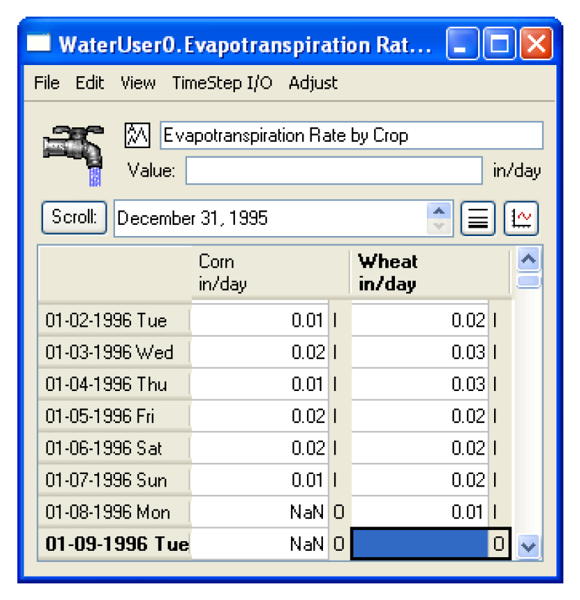
Aggregate Series Slots (Agg Series) are specialized Series Slot that group together one or more Series Slots which are independent of one another. They are used to group together similar series of data. Agg Series slots are essentially multiple individual series of data. The columns of an Agg Series Slot are often referred to as Sub Slots. Figure 5.23 shows the Evapotranspiration Rate by Crop for two different crops, Corn and Wheat.
Figure 5.23
Configuration
Following are configuration options specific to Agg Series Slots. See Configure Slot Dialog for details on general configuration. See Configure Slot Dialog Functionality for details on Series Slots.
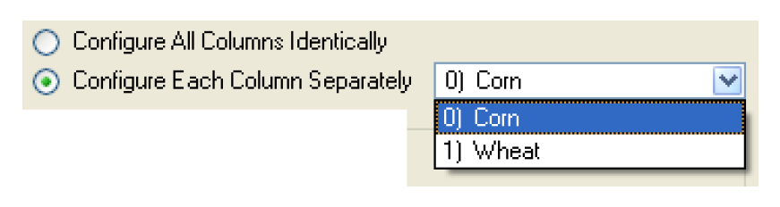
Agg Series slots can be configured such that each column is configured identically or each is configured individually. In the Configuration dialog, there is a toggle to configure the columns identically or separately.
Other Options
Because each column can be configured separately, the time range of each column can be configured to have different start and end dates. The two options allow the columns of the agg series to sync back together:
Max Synch
The Edit, then Max Synch option will synchronize each column to fully encompass the earliest and latest date displayed on any column of the slot. For example, if column 1 goes from Jan. 1, 1999 to June 1, 1999 and column 2 goes from Feb. 2, 1999 to July 23, 1999, a Max Synch will change the range of both columns to be Jan. 1, 1999 to July 23, 1999.
Sync to Column0
The Edit, then Sync to Column0 option will synchronize each to column to match the first column (i.e. column 0). On the previous paragraphs example, a Sync to Column0 will change the range of all columns to be Jan. 1, 1999 to June 1, 1999.
Integer-indexed Series and Agg Series Slots
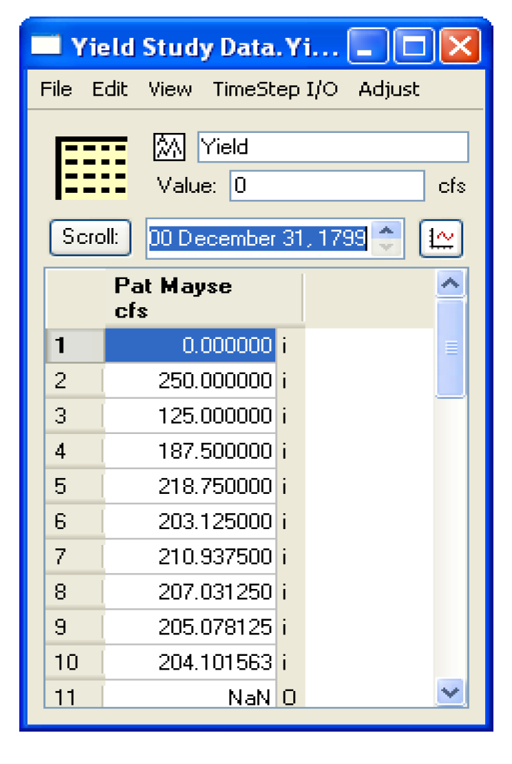
Integer Indexed Series Slots and Integer Indexed Agg Series Slots are specialized types of series slots whose range is associated with their order in the series, rather than with dates. The indices are 1-based; that is, the first value has index 1.
Configuration of Integer Indexed Series Slots is similar to Series Slots, but because the series is incremented by integer, there are a few differences between this type of slot and a standard series slot. See Configure Slot Dialog Functionality for details.
The View menu now has a Series Range menu instead of the standard Timeseries Range menu option. In the Series Range menu (the Configure Series dialog), the Begin, End, and timestep areas are disabled. The user can change the range only by changing the number of values.
Integer Indexed Series slots can be used as a part of the following utilities:
• They are plotted with integer values with units of NONE for the x dimension.
• They can be accessed and set from the RiverWare Policy Language. Integer Indexed Slots are particularly useful in Iterative MRM mode as they can be used to store values for a particular run index.
• They can be displayed on a System Control Table (SCT).
Note: The SCT can either show standard time series or integer indexed series, but not both.
Series Slots With Periodic Input
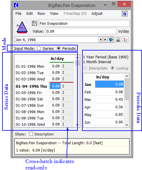
Series Slots with Periodic Input allow you to specify either a series of values or a periodic relationship. You can specify data in one of the following Input Modes:
• Series. The individual time-series values are directly editable in the slot dialog and in an SCT. In this mode, these slots are functionally equivalent to ordinary series slots.
• Periodic. The periodic values are editable and shown in a separate panel. As periodic values are entered, the series values are filled in. As with other periodic slots, you have the choice of several standard periods (e.g. 1 Year, 1 Month, 1 Day), either “irregular” or “regular” intervals within the period, and interpolation or lookup.
Series Slots with Periodic Input behave as ordinary series slots in virtually all ways, including RPL access, plotting, outputs, etc. A minor exception to this is that DMI import operation to these slots is blocked when they are in Periodic input mode.
Series Slots with Periodic Input can be shown in either the Slot Dialog or the Slot Viewer. When the slot is in periodic mode, it opens in its own Slot Dialog. When the slot is in series mode, it opens in the Slot Viewer and there is special ornamentation in the column heading indicating its type, s shown in Figure 5.24. Click the icon to open the slot in its own dialog where you can see the periodic input values.
to open the slot in its own dialog where you can see the periodic input values. Figure 5.24 Screenshot of the Series Slot with Periodic Input in the Slot Viewer.
In general, when switching a Series Slot with Periodic Input from Series to Periodic input mode, the existing series values are lost; they are overwritten with values computed from the periodic input definition. When switching from Periodic to Series input mode, the periodic input values are hidden and become inactive.
The remainder of this section describes creation and editing of these types of slots.
Slot Creation
Series Slots with Periodic Input exist on some engineering objects (particularly the reservoirs) and can be created by the user. From the Object dialog, choose the Slot, then Add Series Slot with Periodic Input menu item.
Slot Configuration
Following are configuration options for this type of slot.
Series Input Mode
Series Slots with Periodic Input start in Series input mode where they appear and behave as ordinary series slots. Figure 5.25 shows Series input mode.
The slots are accessed from RPL using standard series syntax, i.e. by DateTime: Slot[ ] or Slot [E].
Figure 5.25 Screenshot of Series Slot with Periodic Input in both modes
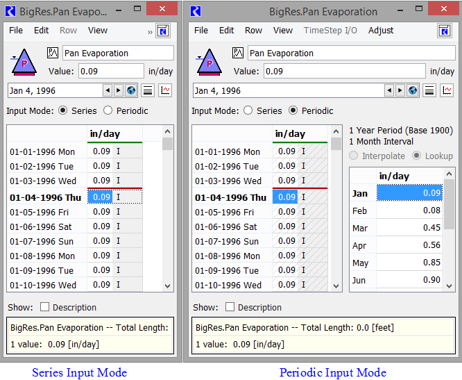
Periodic Input Mode
In Periodic input mode, the series data is shown as read-only (cannot be edited), but an editable periodic data panel is shown to the right (see Figure 5.25). Edits and operations on the periodic values immediately cause a recalculation of the series values—assigned as Inputs except where periodic values are undefined, in which case NaNs (flagged as Outputs) are shown. Series values are computed for the series slot’s currently configured time range.
The periodic configuration is accessible from the View, then Configure Period menu. See Periodic Slots for an explanation of the available period, interval, and data interpolation settings. Use the options in the Row menu to modify the rows of the periodic table.
Although they have periodic data, the slots are accessed from RPL using standard series syntax, i.e. by DateTime: Slot[ ] or Slot [E].
Note: A RPL reference to a value at a timestep outside the time range of the series portion of the slot will return NaN, even when in periodic input mode.
Switching Between Series and Periodic Mode
In general, when switching from Series input mode to Periodic input mode, the series values are overwritten by values computed from the periodic values. When series values are overwritten by periodic data, the you must confirm the warning dialog. No confirmation dialog is shown when switching from Periodic input mode to Series input mode, as there is no loss of data in that change.
Tip: There is a script action Set Series Slot Input Mode that can be used to automate switching modes. See Set Series Slot Input Mode in Automation Tools for more information.
Changing Display Units when in Periodic Mode
In general, when changing the display units of a Series Slot with Periodic Input, the values in a both the Series and entries are converted to the new units. But when in periodic mode and the new or existing unit involves a non-constant timestep length, for example, per month or per year, the series values must be recomputed from the converted periodic values. The recomputed series values will then match the periodic values. A warning message is posted to a dialog box and/or the diagnostics output when this occurs.
Multi Slots
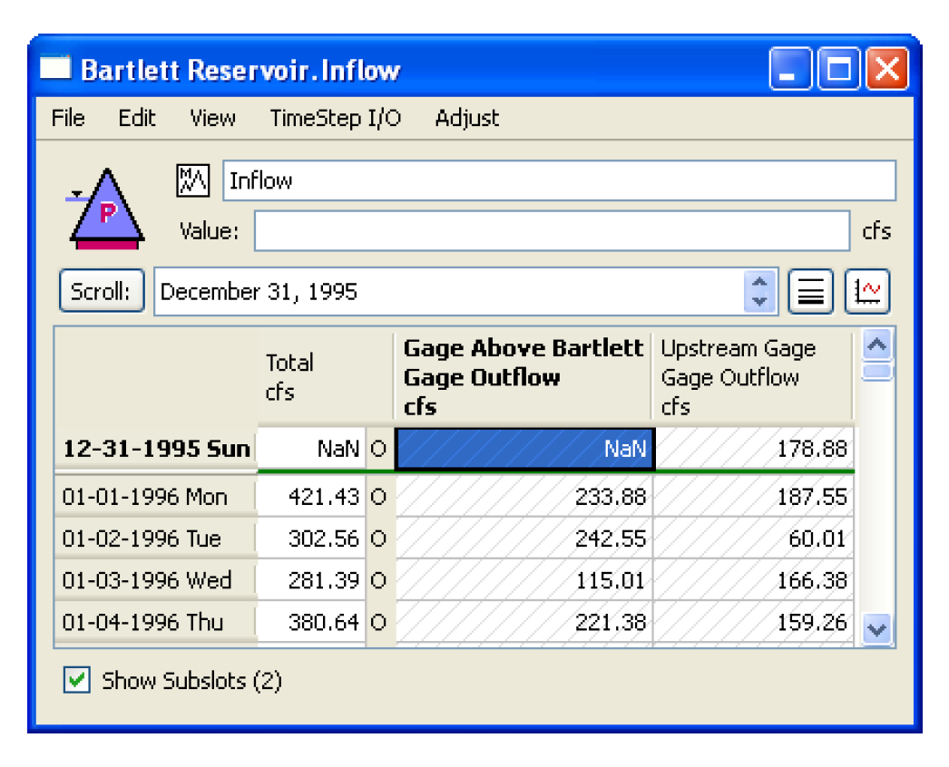
Multi Slots are specialized series slots that automatically sum the values of the slots to which they are linked. In the screenshot, two series slots named Gage Above Bartlett. Gage Outflow and Reach2.Outflow are linked to the Bartlett.Inflow slot. Each of the linked slots appears in a column. The cells for these columns are grey hatched indicating that they are not directly editable from this view. The user should edit these values from the other end of the link. The sum of all linked columns is reported in the Total column. The columns of a Multi Slot are often referred to as Sub Slots. All of the sub slots must have the same unit type and user unit although the other end of the link can have a different user unit, conversion is automatic.
Configuration of Multi Slots is similar to Series Slots; see Configure Slot Dialog Functionality. On Multi Slots there is a toggle at the bottom of the dialog that is used to hide or show the subslots. The checkbox is shown only if the Multi Slot has at least one subslot. It is initialized to OFF if the Multi Slot has exactly one subslot, otherwise, it is initialized to ON. This can be useful for subslots that only have one link, hence it really only represents one series of data.
Table Slots
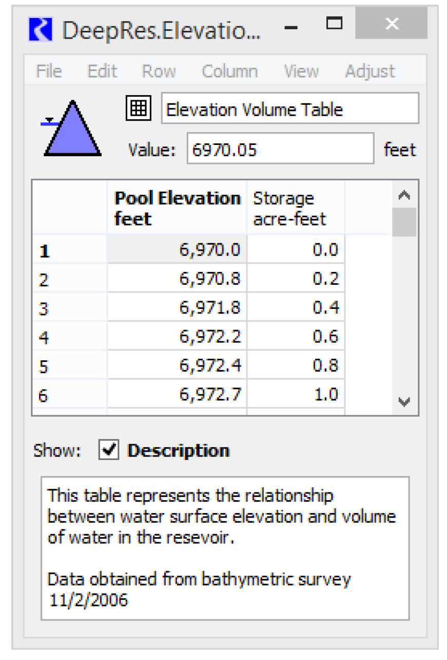
Table Slots are used to store any table of data. They can define a curve (2-Dimensional), a surface (3-Dimensional), or several unrelated sets. A 2-Dimensional table may require monotonically increasing values in its first column, as shown in the Elevation Volume table.
Configuration
See View Menu for details on configuring Table Slots. Each column of the table has both a Label and a Unit (user units are configurable). On simulation slots, the Rows are labeled by number unless defined otherwise. Both columns and rows are zero-based, i.e. the first column is column 0. On custom slots the user is able to change both the Units, Display Format, Column Labels, and Row Labels. Table Slots can be configured such that each column is configured identically or each is configured individually. In the View menu, there is a menu to Configure Columns Identically or separately using the Configure Column menu on the selected column.
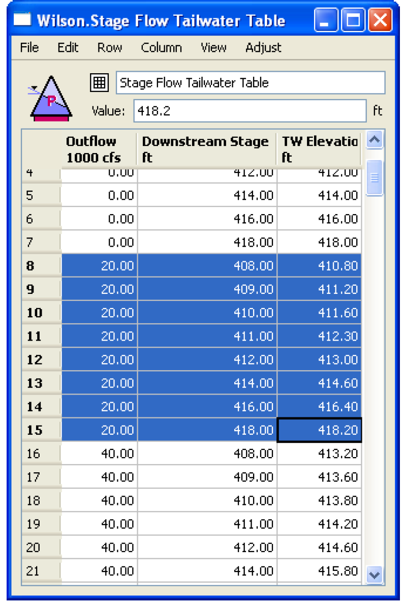
A 3-Dimensional table requires that column 1 contain sets of equal values which increase down the table, and column 2 must contain monotonically increasing values within each set of values from column 1. Column 3 then contains the values to look up for columns 1 and 2. For example, the Stage Flow Tailwater Table is a 3-Dimensional table relating TW Elevation to the independent variables of reservoir Outflow and Downstream Stage. A set where Outflow is equal to 20,000 cfs is highlighted.
Edit Row Configuration
The user is able to change the number of rows in most tables. This is done through the Row menu using the Insert/Append/Delete rows options. Move rows up or down using the Row, then Move Rows menu (Custom Slots only).
Editing Column Configuration
Some Table Slots allow columns to be appended and deleted. This is done to store a variable number of data sets within a single slot. A “block” is defined as the number of columns which must be appended or deleted together. In the case of the Elevation Volume Table, the block size is 2, one column for Pool Elevation and one for Storage (although the user can’t add blocks to this table). When appending or deleting columns from a Table Slot and its dependents, reconfiguring must be done in blocks. The minimum table size is 1 block. The user can change the number of columns using the Set Number of Columns, Append Column, Delete Column, Delete Last Column, and Set Dimensions menu options from the Column menu. Move columns to the right or left using the Column, then Move Columns menu (custom slots only). The Column, then Set Dimensions can also be used to change the number of rows and columns at the same time.
Show Column Sum Row
The user is able to show the sum of the column rows using the View, then Show Column Sum Row menu item. This option adds a special read-only SUM row to the bottom of the column that sums all of the values above (NaNs are assumed to be zero). This feature is especially useful when setting up routing coefficients or factors where the sum of the column must equal 1.0.
Optimization Limits for Data Verification
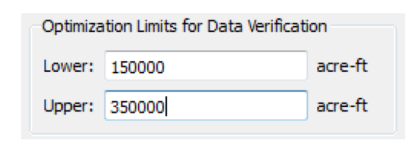
The Table Slot single-column configuration dialog presents an Optimization Limits for Data Verification panel if the column is configured to support optimization checking limits. See Create an Optimization Goal Set in Optimization for details.
Source Slots
Some specific scalars and tables have a “Source” slot. When a slot has a source slot, the values are computed from the source slot’s values. Thus, the destination slot becomes read-only and displays a cross hatch over the data. The slot also provides a note indicating the source slot used to compute the data. The source slot is typically set/un-set at beginning of run, so you must initialize the run to see the read-only status.
Statistical Table Slots
Statistical table slots allow the user to specify a statistical function, such as a flow duration curve, which is computed at the end of a run using the data in specified model slot(s). This statistical analysis data can then be plotting or exported to another application.
This statistical analysis could be computed using Riverware’s existing export or output manager functionality coupled with a third-party analysis application such as Excel. Statistical table slots provides this functionality inside Riverware to allow quick analysis at the end of a run without leaving the Riverware environment.
Creating a Statistical Table Slot
To create a statistical table slot, open the object dialog for a object. From this dialog:
• Select Slot, then Add Statistical Table Slot from the object’s main menu bar.
• Right-click over the slots list and select Add Slot, then Statistical Table Slot from the context menu.
A statistical table slot will be displayed in the slot list with the Slot icon  .
.
. Configuring a Statistical Table Slot
A statistical table slot is configured and viewed using the Statistical Table Slot Dialog. Display this dialog by opening the statistical table slot in the object dialog.
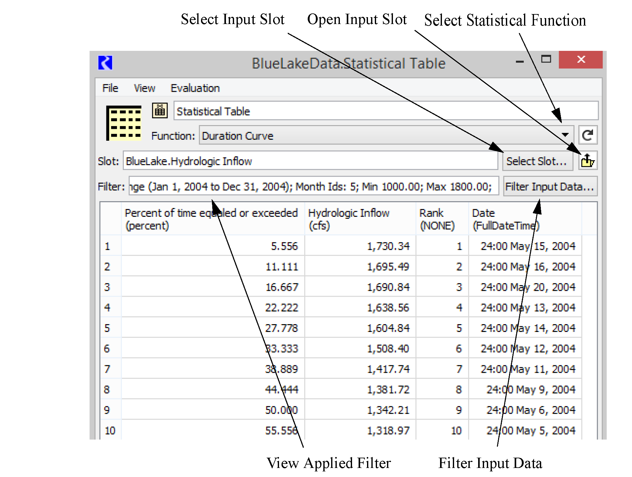
The basic steps in configuring a statistical table slot are:
1. Select the desired statistical function from the Function menu. The functions are described Statistical Functions.
2. Select the input slot for the statistical function by pressing the Select Slot button. A selected input slot can then be opened by pressing the icon next to the Select Slot button.
3. Select any desired filtering of the input data by pressing the Filter Input Data button. Data can be filtered as follows:
– Time Range, select the Run Range (default), full Slot Data Range, or a Specified Range
– Months, choose the desired months
– Values Greater than a Minimum.
– Values Less than a Maximum.
– A specified Number of Largest Values.
Multiple filters can be applied concurrently. A summary of any applied filtering can be viewed on the Statistical Table Slot Dialog in the Filter text window.
4. Specify the display units, scale, and precision for each column in the table by selecting View, then Configure from the dialog’s menu bar.
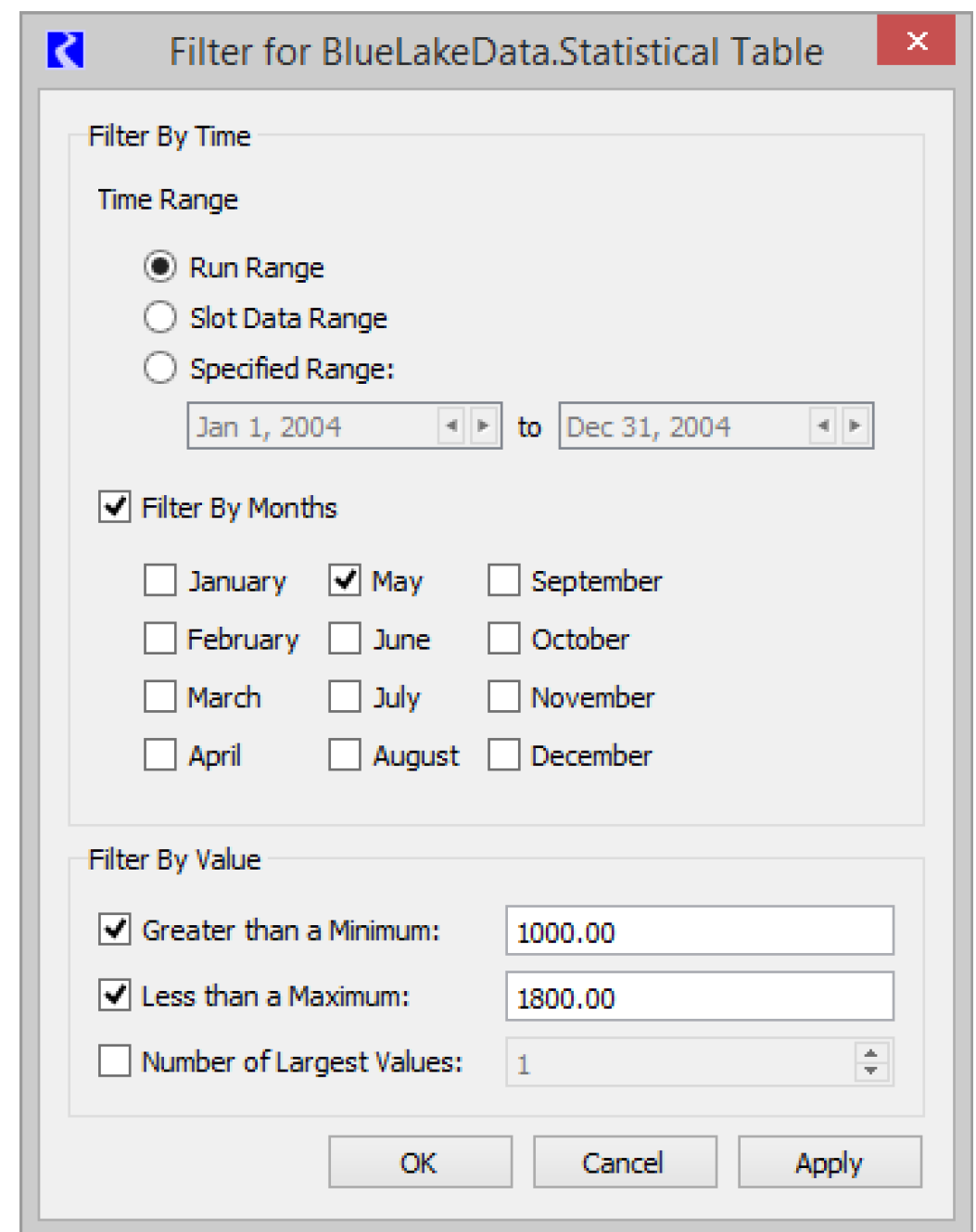
Evaluating a Statistical Table Slot
By default, all statistical table slots will be cleared at the beginning of the run and evaluated at the end of the run.
• To prevent a statistical table slot from being evaluated at the end of the run select Evaluation, then Disabled on the dialog’s menu bar.
The contents of a statistical table slot can also be cleared and evaluated manually.
• To manually evaluate a statistical table slot select Evaluation, then Evaluate (Alt+E) from the slot dialog’s menu bar.
• To manually clear the contents of a statistical table slot select Evaluation, then Clear from the slot dialog’s menu bar.
Analyzing a Statistical Table Slot
Snapshots can be made of statistical slots to easily preserve and compare their values from different runs.
• To create a snapshot of the statistical slot select View, then Snapshot Mgr (Alt+S) from the slot dialog’s menu bar.
• The snapshot manager dialog will be opened and the statistical slot and its input slot will be added to the manager’s slot list if not already present.
• Taking a snapshot creates a data object with copies of all slots that are in the manager’s list.
• To preserve the data, the snapshots of statistical slots have all functionality disabled that could change the values of the data in the slot.
Plotting a Statistical Table Slot
The contents of a statistical table slot can be plotted.
• To plot the contents of the statistical table slot select File, then Plot (Ctrl+P) from the slot dialog’s menu bar.
• If the statistical slot has more than 2 columns, a dialog appears to allow specification of which columns to plot (some functions may present a checkbox option for plotting all the result data columns, for example to plot all duration columns from a value duration function). A typical choice would be percent exceedence probabilities versus values. In this case, the percent exceedences will, by default, be plotted on a probability scale as you would see on normal probability paper. On such a scale, normally distributed values will plot as a straight line.
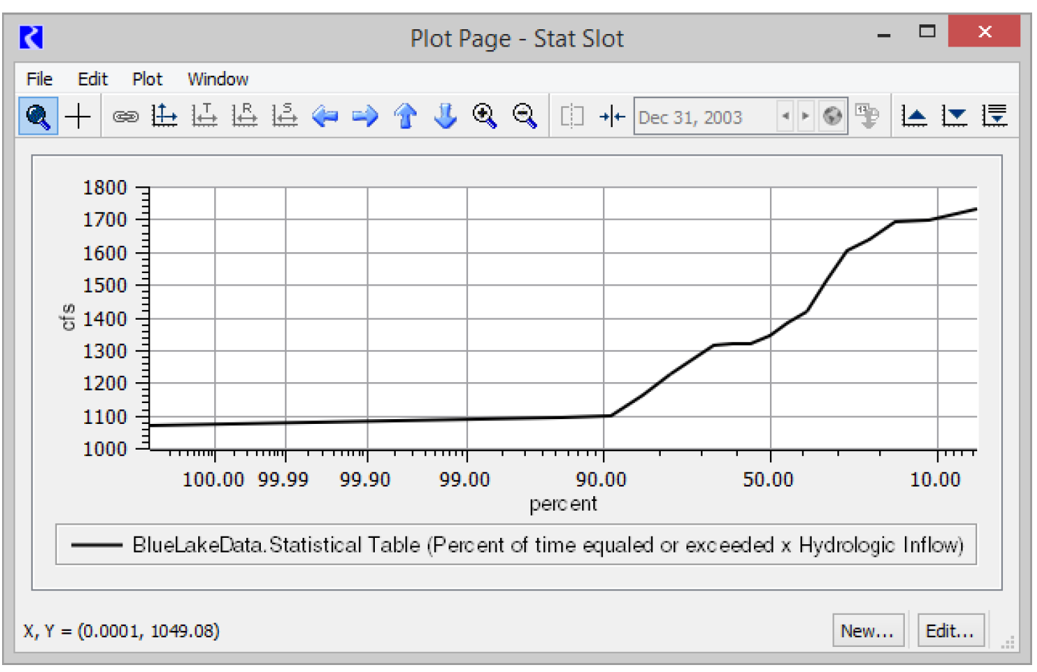
• If desired, the probability axis can be changed to a linear scale by selecting Edit, then Axis Configuration from the plot dialog’s menu bar, then choosing the X-Axis and changing the toggle.
• The axes of the generated plot can also be configured to be logarithmic by selecting Edit, then Axis Configuration from the plot dialog’s menu bar. This can be used, for example, to plot a log-normal representation of the data.
• The configuration of the plot can be saved for quick access by using either the output manager or the File, then Save As option on the plot dialog.
A statistical slot can be plotted with all of its snapshots.
• To plot the contents of the statistical table slot along with all of its snapshots, select File, then Plot with Snapshots (Alt+P) from the slot dialog’s menu bar.
• If the statistical slot has more than 2 columns, a dialog appears to allow specification of which columns to plot (some functions may provide a checkbox option to plot all the result data columns). The selections are used for the slot as well as for all the snapshots.
• The slot’s data and the data in all of its snapshots are plotted on the same graph to allow for an easy visual comparison.
• The axes of the generated plot can be configured to logarithmic scale by selecting Edit, then Axis Configuration from the plot dialog’s menu bar.
• The configuration of this plot can be saved for quick access by using either the output manager or the File, then Save As option on the plot dialog.
User data input to a table slot can be plotted with a statistical slot.
• Add a table slot by selecting Slot, then Add Table Slot menu.
• A dialog will appear asking for the number of rows and columns you want in your table slot. You will probably want at least two columns to plot the slot.
• The new table slot with a default name will appear in the slot list. Double-click the new table slot in this list to bring up the table slot’s dialog.
• Select View, then Column Labels from the table slot’s dialog. Give the columns heading names in the new dialog that comes up and select OK.
• Now select View, then Configure from the table slot’s dialog. Assign Unit Type and User Units to your columns by using the Configure Each Column Separately option.
• Enter the desired data into the cells of the table slot’s dialog.
• From a plot of your statistical slot, select Data, then Add Table Curve from the plot’s menu bar.
• From the resulting Curve Configuration dialog, select the Select Table Slot button and select the table slot you created above.
• The Curve Configuration dialog will allow you to select what columns you wish to plot on the x and y axes of the plot along with line styles and formats.
• Selecting OK on the Curve Configuration dialog will then add your user input data from the table slot onto the plot with the statistical slot.
The contents of the statistical table slot can also be exported to a text file for analysis using an external tool.
• To export the contents of the table slot select File, then Export (Display Precision) or File, then Export (Model Precision) from the slot dialog’s menu bar.
Statistical Functions
The following statistical functions are provided on RiverWare’s statistical table slots.
Duration Curve
Duration Curve | |
|---|---|
Input Slot(s) | 1 series slot |
Column 0 | Label: Percent of time equaled or exceeded Unit Type: Fraction |
Column 1 | Label: [Name of input slot] Unit Type: [Unit type of input slot] |
Column 2 | Label: Rank Unit Type: None |
Column 3 | Label: Date Unit Type: DateTime |
Algorithm | 1. Filter the input data from the input slot per the user’s specifications. 2. Sort all n resulting values in decreasing order. 3. Assign a rank to each sorted item from 1 to n. The rank of the item is m. For the largest slot value, m=1. For the smallest slot value, m = n. 4. Compute the statistical exceedence percentage value (P) for each item using the formula: P = m / n. 5. The final output is the list of: P, the slot values in sorted descending order, rank, and date of the values. |
Annual Max Frequency Curve
Annual Max Frequency Curve | |
|---|---|
Input Slot(s) | 1 series slot |
Column 0 | Label: Max exceedence frequency in percent of years Unit Type: Fraction |
Column 1 | Label: [Name of input slot] Unit Type: [Unit Type of input slot] |
Column 2 | Label: Rank Unit Type: None |
Column 3 | Label: Date Unit Type: DateTime |
Algorithm | 1. Filter the input data from the input slot per the user’s specifications. 2. Create a list of the maximum annual values for each year within the resulting data. 3. Sort all n annual values in decreasing order. 4. Assign a rank to each sorted item from 1 to n. The rank of the item is m. For the largest slot value, m=1. For the smallest slot value, m=n. 5. Compute the statistical exceedence percentage value (P) for each item using the formula:  ; Pn = 1 - P1 ; P for all others interpolated between these two based on rank. ; Pn = 1 - P1 ; P for all others interpolated between these two based on rank.6. The final output is the list of: P, the max annual values in sorted descending order, rank, and date of the value. |
Annual Min Frequency Curve
Annual Min Frequency Curve | |
|---|---|
Input Slot(s) | 1 series slot |
Column 0 | Label: Min exceedence frequency in percent of years Unit Type: Fraction |
Column 1 | Label: [Name of input slot] Unit Type: [Unit Type of input slot] |
Column 2 | Label: Rank Unit Type: None |
Column 3 | Label: Date Unit Type: DateTime |
Algorithm | 1. Filter the input data from the input slot per the user’s specifications. 2. Create a list of the minimum annual values for each year within the resulting data. 3. Sort all n annual values in increasing order. 4. Assign a rank to each sorted item from 1 to n. The rank of the item is m. For the largest slot value, m=1. For the smallest slot value, m=n. 5. Compute the statistical exceedence percentage value (P) for each item using the formula:  ; Pn = 1 - P1 ; P for all others interpolated between these two based on rank. ; Pn = 1 - P1 ; P for all others interpolated between these two based on rank.6.The final output is the list of: P, the min annual values in sorted ascending order, rank, and date of the value. |
Annual Avg Frequency Curve
Annual Avg Frequency Curve | |
|---|---|
Input Slot(s) | 1 series slot |
Column 0 | Label: Avg exceedence frequency in percent of years Unit Type: Fraction |
Column 1 | Label: [Name of input slot] Unit Type: [Unit Type of input slot] |
Column 2 | Label: Rank Unit Type: None |
Column 3 | Label: Date Unit Type: DateTime |
Algorithm | 1. Filter the input data from the input slot per the user’s specifications. 2. Create a list of the average annual values for each year within the resulting data. 3. Sort all n annual values in decreasing order. 4. Assign a rank to each sorted item from 1 to n. The rank of the item is m. For the largest slot value, m=1. For the smallest slot value, m=n. 5. Compute the statistical exceedence percentage value (P) for each item using the formula:  ; Pn = 1 - P1 ; P for all others interpolated between these two based on rank. ; Pn = 1 - P1 ; P for all others interpolated between these two based on rank.6. The final output is the list of: P, the avg annual values in sorted descending order, rank, and date of the value. |
Monthly Maximums By Year
Monthly Maximums By Year | |
|---|---|
Input Slot(s) | 1 series slot |
Column 0 | Label: Year Unit Type: DateTime |
Columns 1 - 12 | Label: [Month] Max Unit Type: [Unit Type of input slot] |
Column 13 | Label: Annual Max Unit Type: [Unit Type of input slot] |
Final Rows | Labels: Maximum, Minimum, Average (of the columns) Unit Type: [Unit Type of input slot] |
Algorithm | 1. Filter the input data from the input slot per the user’s specifications. 2. Iterate the data and track and save the maximum value for each month and for each year. 3. Generate average maximum values for each month across all years and for the annual maximum across all years. 4. The final output is a row for each year and final rows for maximums, minimums, and averages across all the years. Columns are the date for the year, a column for each month’s maximum, and an annual maximum column. |
Monthly Minimums By Year
Monthly Minimums By Year | |
|---|---|
Input Slot(s) | 1 series slot |
Column 0 | Label: Year Unit Type: DateTime |
Columns 1 - 12 | Label: [Month] Min Unit Type: [Unit Type of input slot] |
Column 13 | Label: Annual Min Unit Type: [Unit Type of input slot] |
Final Rows | Labels: Maximum, Minimum, Average (of the columns) Unit Type: [Unit Type of input slot] |
Algorithm | 1. Filter the input data from the input slot per the user’s specifications. 2. Iterate the data and track and save the minimum value for each month and for each year. 3. Generate average minimum values for each month across all years and for the annual minimum across all years. 4. The final output is a row for each year and final rows for maximums, minimums, and averages across all the years. Columns are the date for the year, a column for each month’s minimum, and an annual minimum column. |
Monthly Averages By Year
Monthly Averages By Year | |
|---|---|
Input Slot(s) | 1 series slot |
Column 0 | Label: Year Unit Type: DateTime |
Columns 1 - 12 | Label: [Month] Avg Unit Type: [Unit Type of input slot] |
Column 13 | Label: Annual Avg Unit Type: [Unit Type of input slot] |
Final Rows | Labels: Maximum, Minimum, Average (of the columns) Unit Type: [Unit Type of input slot] |
Algorithm | 1. Filter the input data from the input slot per the user’s specifications. 2. Iterate the data and calculate and save the average value for each month and for each year. 3. Generate averages from the average values for each month across all years and for the annual average value across all years. 4. The final output is a row for each year and final rows for maximums, minimums, and averages across all the years. Columns are the date for the year, a column for each month’s average, and an annual average column. |
Monthly Totals By Year
Note: Totals generated by this function may not make sense for some slots (i.e, flow or storage).
Monthly Totals By Year | |
|---|---|
Input Slot(s) | 1 series slot |
Column 0 | Label: Year Unit Type: DateTime |
Columns 1 - 12 | Label: [Month] Tot Unit Type: [Unit Type of input slot] |
Column 13 | Label: Annual Tot Unit Type: [Unit Type of input slot] |
Final Rows | Labels: Maximum, Minimum, Average (of the columns) Unit Type: [Unit Type of input slot] |
Algorithm | 1. Filter the input data from the input slot per the user’s specifications. 2. Iterate the data and track and save the total value for each month and for each year. 3. Generate average total values for each month across all years and for the annual total across all years. 4. The final output is a row for each year and final rows for maximums, minimums, and averages across all the years. Columns are the date for the year, a column for each month’s total, and an annual total column. |
Monthly Medians By Year
Monthly Medians By Year | |
|---|---|
Input Slot(s) | 1 series slot |
Column 0 | Label: Year Unit Type: DateTime |
Columns 1 - 12 | Label: [Month] Med Unit Type: [Unit Type of input slot] |
Column 13 | Label: Annual Med Unit Type: [Unit Type of input slot] |
Final Rows | Labels: Maximum, Minimum, Average (of the columns) Unit Type: [Unit Type of input slot] |
Algorithm | 1. Filter the input data from the input slot per the user’s specifications. 2. For each set of data for that month and year, sort the data and select the “middle” value, If there are an even number of values, the median is the mean of two middle values. 4. The final output shows: • A row for each year and a column for each month. • The final column is the median of all values in the year, not just the values for that row. • The final rows show the maximums, minimums, and means across all the years of the median data in the column. |
Partial Duration Max Frequency Curve
Partial Duration Max Frequency Curve | |
|---|---|
Input Slot(s) | 1 series slot |
Column 0 | Label: Max exceedence frequency in percent Unit Type: Fraction |
Column 1 | Label: [Name of input slot] Unit Type: [Unit Type of input slot] |
Column 2 | Label: Rank Unit Type: None |
Column 3 | Label: Date Unit Type: DateTime |
Algorithm | 1. Filter the input data from the input slot per the user’s specifications. 2. If user has specified a base value, use it in the call to the partial duration calculation and present all the results generated. 3. If not a user-supplied base value, sort the input values in decreasing order and assume a base equal to the value at position (number of years of input data plus one). Make successive calls to the partial duration calculation with decreasing base values until the number of results equals or exceeds the number of years of data in the input slot. 4. The partial duration calculation tabulates the largest values that are greater than the base value, which are separated by events less than the base value. 5. Sort all n result values in decreasing order. 6. Assign a rank to each sorted item from 1 to n. The rank of the item is m. For the largest slot value, m=1. For the smallest slot value, m=n. 7. Compute the statistical exceedence percentage value (P) for each item. For the top half of items, use the formula:  ; Pn = 1 - P1 ; P for all others in the top half are interpolated between these two based on rank. For the bottom half of items, use the formula: ; Pn = 1 - P1 ; P for all others in the top half are interpolated between these two based on rank. For the bottom half of items, use the formula: 8. The final output is the list of: P, the max partial duration values in sorted descending order, rank, and date of the value. |
Partial Duration Min Frequency Curve
Partial Duration Min Frequency Curve | |
|---|---|
Input Slot(s) | 1 series slot |
Column 0 | Label: Min exceedence frequency in percent Unit Type: Fraction |
Column 1 | Label: [Name of input slot] Unit Type: [Unit Type of input slot] |
Column 2 | Label: Rank Unit Type: None |
Column 3 | Label: Date Unit Type: DateTime |
Algorithm | 1. Filter the input data from the input slot per the user’s specifications. 2. If user has specified a base value, use it in the call to the partial duration calculation and present all the results generated. 3. If not a user-supplied base value, sort the input values in increasing order and assume a base equal to the value at position (number of years of input data plus one). Make successive calls to the partial duration calculation with increasing base values until the number of results equals or exceeds the number of years of data in the input slot. 4. The partial duration calculation tabulates the smallest values that are less than the base value, which are separated by events greater than the base value. 5. Sort all n result values in increasing order. 6. Assign a rank to each sorted item from 1 to n. The rank of the item is m. For the largest slot value, m=1. For the smallest slot value, m=n. 7. Compute the statistical exceedence percentage value (P) for each item. For the top half of items, use the formula:  ; Pn = 1 - P1 ; P for all others in the top half are interpolated between these two based on rank. For the bottom half of items, use the formula: ; Pn = 1 - P1 ; P for all others in the top half are interpolated between these two based on rank. For the bottom half of items, use the formula: 8. The final output is the list of: P, the min partial duration values in sorted ascending order, rank, and date of the value. |
Value Duration Max Frequency Curve
Value Duration Max Frequency Curve | |
|---|---|
Input Slot(s) | 1 series slot |
Column 0 | Label: Max exceedence frequency in percent of years Unit Type: Fraction |
Columns 1 - N | Label: [Duration represented by column] Unit Type: [Unit Type of input slot] |
Algorithm | 1. Filter the input data from the input slot per the user’s specifications. 2. Determine the durations to use in calculation based on timestep of input slot. Currently only implemented for day (1, 2, 3, 5, 7, 19, 15, 60, 90 and 365 day) and month (1, 2, 3, 4, 6 and 12 month) 3. Loop for each duration. 4. For each year, average the slot values over the duration starting with timestep 1, then starting with timestep 2, etc. to generate a set of values over this duration for the year. Take the maximum of this set of values and record this as the single result for the year. 6. Sort all the result values (one for each year) in decreasing order and present as a column of results for this duration. 7. Move on to the next duration. 4. Assign a rank to each row of results from 1 to n. 5. Compute the statistical exceedence percentage value (P) for each row using the formula:  ; Pn = 1 - P1 ; P for all others interpolated between these two based on row rank. ; Pn = 1 - P1 ; P for all others interpolated between these two based on row rank.6. The final output is the list of: P and a column of results for each duration used. |
Value Duration Min Frequency Curve
Value Duration Min Frequency Curve | |
|---|---|
Input Slot(s) | 1 series slot |
Column 0 | Label: Min exceedence frequency in percent of years Unit Type: Fraction |
Columns 1 - N | Label: [Duration represented by column] Unit Type: [Unit Type of input slot] |
Algorithm | 1. Filter the input data from the input slot per the user’s specifications. 2. Determine the durations to use in calculation based on timestep of input slot. Currently only implemented for day (1, 2, 3, 5, 7, 19, 15, 60, 90 and 365 day) and month (1, 2, 3, 4, 6 and 12 month) 3. Loop for each duration. 4. For each year, average the slot values over the duration starting with timestep 1, then starting with timestep 2, etc. to generate a set of values over this duration for the year. Take the minimum of this set of values and record this as the single result for the year. 6. Sort all the result values (one for each year) in increasing order and present as a column of results for this duration. 7. Move on to the next duration. 4. Assign a rank to each row of results from 1 to n. 5. Compute the statistical exceedence percentage value (P) for each row using the formula:  ; Pn = 1 - P1 ; P for all others interpolated between these two based on row rank. ; Pn = 1 - P1 ; P for all others interpolated between these two based on row rank.6. The final output is the list of: P and a column of results for each duration used. |
Value Duration Avg Frequency Curve
Value Duration Avg Frequency Curve | |
|---|---|
Input Slot(s) | 1 series slot |
Column 0 | Label: Avg exceedence frequency in percent of years Unit Type: Fraction |
Columns 1 - N | Label: [Duration represented by column] Unit Type: [Unit Type of input slot] |
Algorithm | 1. Filter the input data from the input slot per the user’s specifications. 2. Determine the durations to use in calculation based on timestep of input slot. Currently only implemented for day (1, 2, 3, 5, 7, 19, 15, 60, 90 and 365 day) and month (1, 2, 3, 4, 6 and 12 month) 3. Loop for each duration. 4. For each year, average the slot values over the duration starting with timestep 1, then starting with timestep 2, etc. to generate a set of values over this duration for the year. Take the average of this set of values and record this as the single result for the year. 6. Sort all the result values (one for each year) in decreasing order and present as a column of results for this duration. 7. Move on to the next duration. 4. Assign a rank to each row of results from 1 to n. 5. Compute the statistical exceedence percentage value (P) for each row using the formula:  ; Pn = 1 - P1 ; P for all others interpolated between these two based on row rank. ; Pn = 1 - P1 ; P for all others interpolated between these two based on row rank.6. The final output is the list of: P and a column of results for each duration used. |
Table Series Slot
Table Series Slots are a specialized table slot whose rows correspond to timesteps. This slot contains limited timeseries functionality thus making it more efficient than Series Slots. It was created as a way to efficiently write and/or read large amounts of data. Table Series Slots are primarily used within object user methods such as the Muskingum Cunge hydraulic routing methods. These types of slots cannot be created as custom slots.
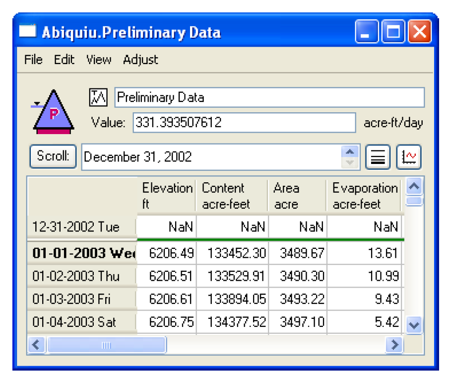
Periodic Slots
Periodic slots are tables used to represent periodic data which repeats at regular time interval. An example might be a set of evaporation coefficients for a reservoir. The rate of evaporation varies with such factors as temperature and wind speed, factors which vary seasonally. It is natural to assume that this variation is the same for each year. If this sort of data were entered into a series slot, then the same data would need to be repeated every year. This would be impractical and inconvenient for the user. On the other hand, if this data were entered in to a table slot, then the data would lose the time element associated with each value. This would make it difficult to look up or interpolate values with respect to time. The periodic slot solves both of these problems.
Figure 5.26
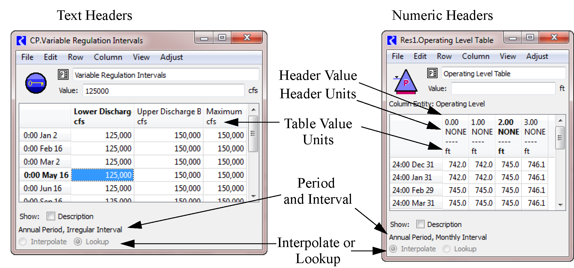
Configuration Options
Periodic slots are configured in the same way as other slots, by using the View, then Configure menu.
The upper left portion of the Configure Slot dialog, under the Period section, is used to set the period and interval of the periodic slot. The period can range from 6-hours to several years while the interval depends on the period selected. If the period required is more than 1 year, the Qty value should be modified from 1 to the number of years and the Base year—the first year in the period—should be defined. Base year can be specified explicitly or symbolically using the menu. If not specified explicitly, they must be edited to become valid, e.g. by replacing the “N” with a nonnegative integer or “YYYY” with a year. Text below the editor field indicates the actual year or indicates the entry is invalid. The Help button provides more information on legal DateTimes.
Also notice the checkbox next to Regular Interval. If the data interval is not a consistent length of time, the user can clear this option and the periodic slot would then have an irregular interval. The user is then free to configure the rows/timesteps in any fashion. See Display of Dates for details.
The Data Access section located in the upper right portion of the Configure Slot dialog is used to specify whether or not data should be interpolated or looked up directly when accessing the table at a time that is not specifically listed as a row label. For example, the monthly data is shown for the beginning of each month. If we’re in the middle of the month, should we use that same piece of data, or should we interpolate between the two months? This is a question that would need to be answered on a per model basis, however, the default behavior is a direct lookup.
Note: Slots configured to Lookup use the value in the row that has a DateTime less than or equal to the desired DateTime, and the DateTime in the next row is greater than the desired DateTime. Slots configured to Interpolate, perform a linear interpolation using values whose rows’ DateTimes bound the desired DateTime.
Columns can be added/deleted by selecting a column and using the Column menu.
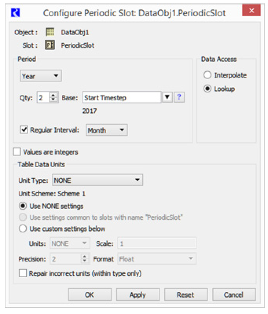
Display of Dates
The rows of a periodic slot represent dates and are displayed differently if the interval is Regular or Irregular. This distinction in dates is described below.
Regular Intervals
Regular Interval periodic slots only show enough information to identify the date. The display is different if the slot is configured to Lookup or Interpolate. When the slot is configured to Lookup, the rows only show the part of the date the changes from one row to the next. Thus, if it is a 1 Month interval, only the month is shown not the hour or day. If it is a 1 Day interval with a 1 Year period, only the day number is shown.
For periodic slots that are configured to Interpolate, the date represents an instant in time that corresponds to the end of a timestep. Thus, for a 1 Month interval, the dates are 24:00 Dec 31, 24:00 Jan1, etc.
Note: Feb 29 is shown in this case but actually behaves as though it is 0:00 March 1.
shows screenshots of a periodic slot that has a Regular Interval of 1 Month.
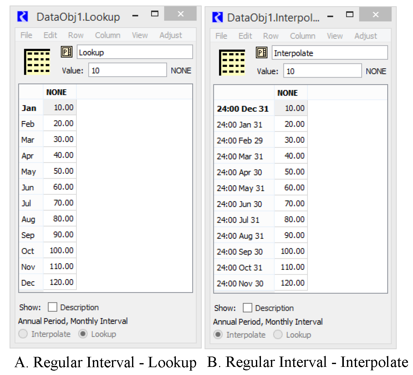
When a new periodic slot (Text Headers) is added, this is how it appears. The following table shows some sample results for the slots shown using the specified DateTime.
For Regular Intervals, the user cannot add or delete rows. The slot must be converted to an Irregular Interval first.
DateTime | A.Regular Interval: Lookup | B. Regular Interval: Interpolate |
|---|---|---|
24:00 January 13, 2001 | 10 | 14.2 |
24:00 February 23, 2003 | 20 | 28.2 |
24:00 October 21, 2009 | 100 | 106.8 |
Irregular Intervals
For Irregular Intervals, the timestep displayed is an instant in time. The screenshot shows the same slots above converted to an Irregular Interval. Because they have the same rows (displayed differently), the A slots would behave the same and the B slots would behave the same.
The user can add or delete rows from periodic slots with an Irregular Interval using the Row menu.
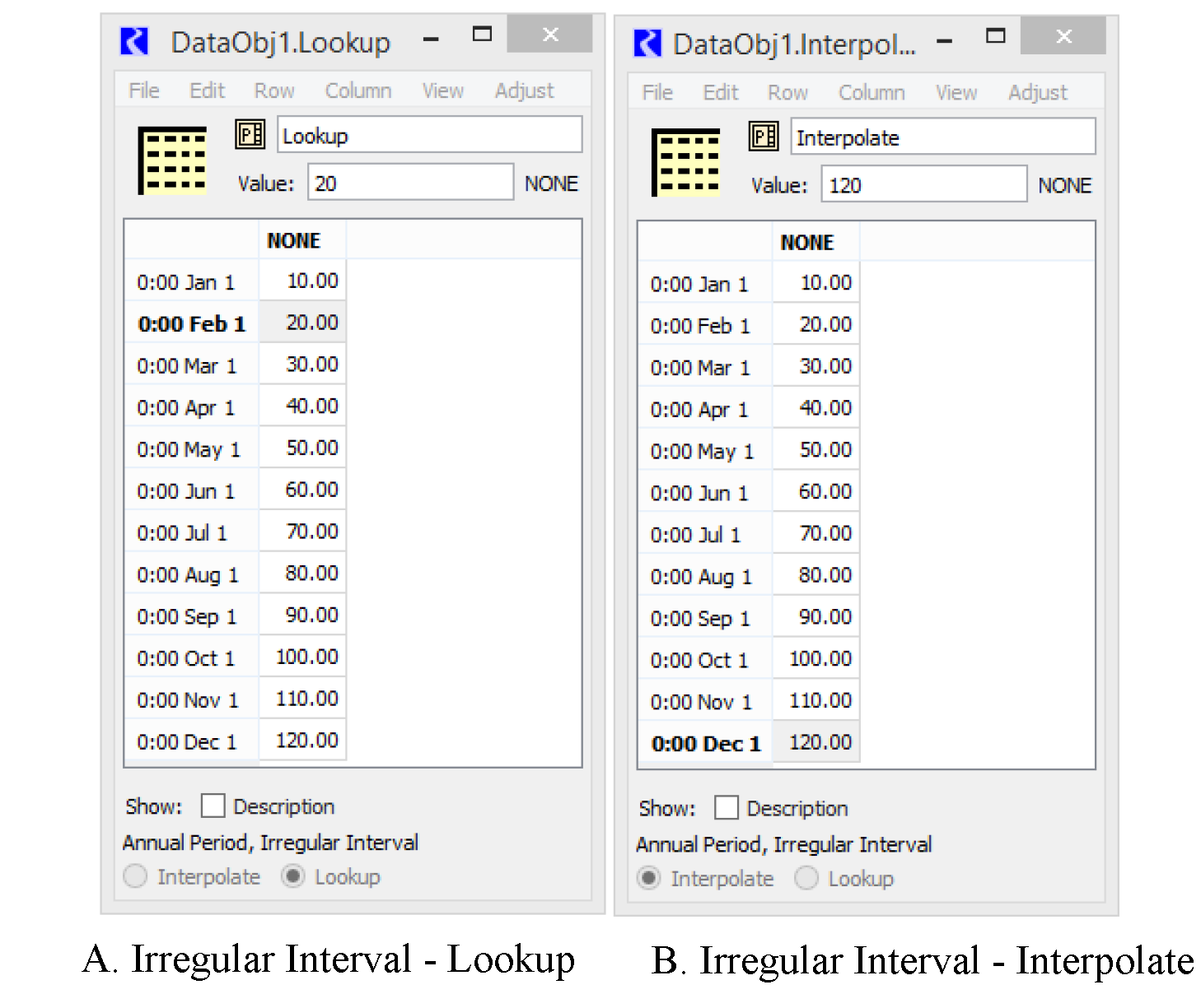
Headers
The user can create the following types of periodic slots:
• With text headers for the columns
• With numeric headers for the columns
Text Headers
In this mode, the periodic slot simply contains columns of data that may or may not be related. There can be no interpolation across columns.To add a periodic slot with Text Headers:
1. Append a periodic slot by selecting Slots, then Add Periodic Slot, Text Headers.
2. If the columns are to be accessed using text, select Column, then Set Column Label to add a text header to each of the columns.
Columns of Periodic Slots with Text Headers can be rearranged using the Column, then Move Columns menu (custom slots only).
Numeric Headers
Consider a periodic slot containing loss coefficients. The periodic slot may contain loss coefficients that vary not only with time, but also with flow rate in a reach. RiverWare could identify which coefficient to use by indexing the table row using the current time step and the table columns using a flow rate. The user could specify as many columns as necessary to sufficiently describe the variation of loss coefficients as a function of flow rate. The periodic slot’s Column Units would be configured to be flow, perhaps with units of 1000 cfs.
To add a periodic slot with Numeric Headers:
1. Append a periodic slot by selecting Slots, then Add Periodic Slot, Numeric Headers.
2. Select View, then Configure to configure the periodic slot
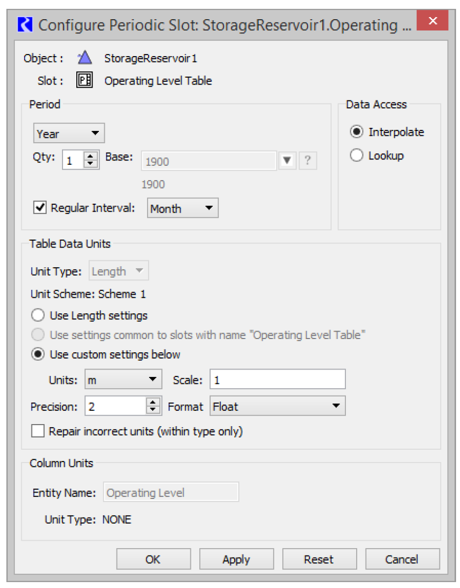
The dialog has a Column Units section. This may be useful if the columns are indexed using numeric header values and the values have some physical (not simply descriptive) significance. The unit specification uses the unit type settings for the active Unit Scheme; see Editing Attributes for details.
The periodic slot can be used backwards to work from the table values and date outward to define a value associated with the column(s). For example, suppose the periodic slot defines the various pools or phases in a reservoir. The conservation pool may be defined as phase 1 with the first column containing pool elevations defining the conservation pool throughout the year. This first column would have a header of 1.0, meaning phase 1. The flood pool may be phase 2.0 with a second column using 2.0 as its header. The surcharge pool may be phase 3.0, etc. Knowing the pool elevation at a given time, the periodic slot can be used to determine the current phase. Interpolating across columns, this outward lookup may determine that the current phase is 2.5 for a given pool elevation and date, meaning pool is halfway from the bottom of flood pool to the bottom of the surcharge pool.
Referencing Periodic Slots in RPL
In RPL, periodic slots are referenced using the Slot[E, E] syntax. Like other tables, this is a row by column reference. But, because it is a periodic slot, the row is a DateTime: Slot[<DateTime>, E]. When referenced in RPL, the configuration of the slot will be used when accessing dates that are “between rows”. That is, it will either interpolate or look up depending on the slot’s configuration.

For periodic slots with text headers, the column specification is a text string matching a column or the zero-based column index. For periodic slots with numeric headers, the column specification is a numeric value with units. You can specify any number that falls within the min and max column values. That is, you don’t have to specify an exact column’s value, but can use numeric values that are “between columns” and it will linearly interpolate for you. For example, the slot shown in Table 5.2 represents low flows that are based on reservoir levels. It is configured to lookup.
5000 ft | 5010 ft | |
|---|---|---|
Jan. 1 | 10 cfs | 20 cfs |
Feb 1 | 40 cfs | 60 cfs |
March 1 | 60 cfs | 80 cfs |
In RPL, to reference this slot on January 15 for reservoir elevation 5002ft, the following would be used:
Slot[@“January 15,2011”, 5002 ft]
It would return the following:
12 cfs
Scalar Slots
Scalar slots represent a single value. Configuration options include units and display format. Scalar slots are used only for input data parameters. See View Menu for details on configuring slots, including Scalar Slots.
Scalar Slot Dialog and Slot Viewer (Scalar)
Scalar slots open by default in the Slot Viewer (Scalar) but you can show them in their own Open Slot dialog box by undocking them. Figure 5.27 highlights the differences between the individual Slot dialog and the Slot Viewer. Following the figure are FAQs that compare and contrast the two interfaces.
Figure 5.27 Screenshot comparing a scalar slot dialog box and the slot viewer
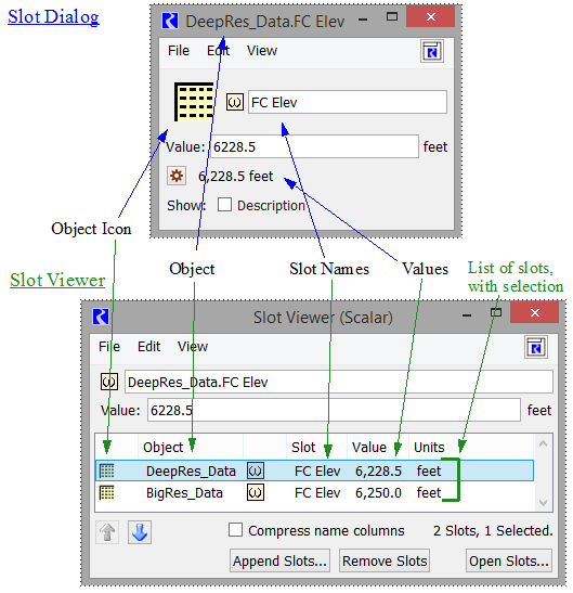
How many of each dialog are there?
There is one Slot Viewer (Scalar) per model. There can be many slot dialogs.
Which slots will open in the Slot Viewer (Scalar)?
The Slot Viewer (Scalar) shows scalar slots and 1X1 table slots. Series slots are displayed in their own slot viewer described in Slot Dialog and Slot Viewer
All other types of slots (Periodic and Table) are shown in their own Slot dialog.
How do I get back to the slot viewer if it gets minimized or hidden?
The workspace has a Slot Viewers button/menu in the lower right. Select the desired Slot Viewer when it has been minimized or hidden behind other dialogs. But, remember that if the Slot Viewers have been closed or all slots are removed from it, the Slot Viewer no longer exists and the button is disabled.
Can the two types of dialogs interact?
From the Slot Viewer, you can undock the scalar slot using the File and then Undock menu or right-click options to create its own dialog box. You can then drag the slot icon on the scalar slot and drop it on the Slot Viewer (Scalar) to redock it.
Where can I find more information?
Slot Viewer (Scalar)
The Slot Viewer (Scalar) provides a compact display of multiple scalar slots simultaneously. It is the default view for scalar data in the same way that the Slot Viewer is the default view for time series slots. The Slot Viewer (Scalar) supports the following functionality:
• Display multiple scalar slots and 1x1 table slots in a compact tabular format.
• Easily add and remove slots from the viewer.
• Edit a slot's value directly without first opening its slot dialog box.
• Easily open a slot's dialog box or configuration dialog box.
• Copy and paste slot values.
The Slot Viewer (Scalar) contains a table of slots containing scalar data, a set of controls to display and manipulate the selected slot's data, and a standard menu bar. Figure 5.28 shows the Slot Viewer (Scalar) containing a variety of slots and data types.
Figure 5.28 Screenshot of the Scalar Data Viewer with a numeric-valued slot selected.
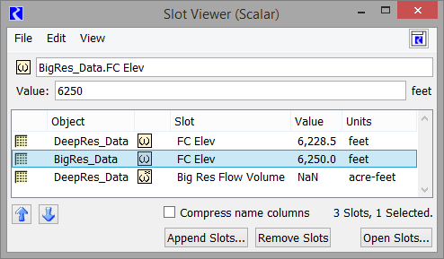
The following operations are not supported on the Slot Viewer (Scalar), but are supported from the Scalar Slot dialog:
• Import and/or export the value
• Plot the value
• Clear the value from a menu. You can type NaN in the edit field to clear the value.
• Add or show the slot description
Open the Scalar Slot dialog first to perform these operations.
Scalar Slot Dialog Functionality
The scalar slot dialog, i.e. the Open Slot for Scalar slots, was the original interface and previously the only way to view and configure scalar slots. Figure 5.29 shows a view of the dialog and all of the pieces. This dialog shows one slot and one scalar value. Use the View and then Configure menu or button to change the settings of the slot. The configuration settings are similar to the general open slot described in Configure Slot Dialog.
Figure 5.29 Annotated screenshot of Scalar Slot dialog
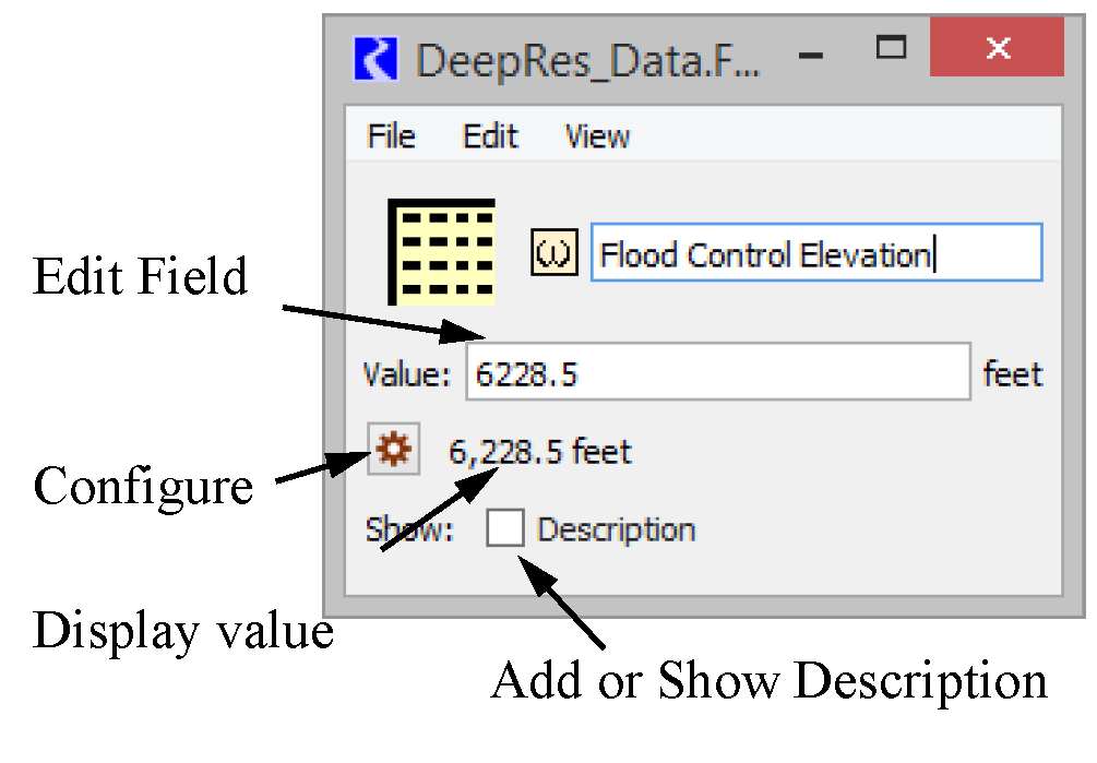
The menu bar operations also support the ability to:
• Dock the slot in the Slot Viewer (Scalar)
• Import and/or export the value
• Plot the scalar value
• Clear the value. You can also type NaN in the edit field to clear the value.
• Undo and redo of value edits
• Configure the slot settings
• Add or show the slot description
Some specific scalars and tables have a Source slot. When a slot has a source slot, the values are computed from other slot values. Thus, it becomes read-only and displays a cross hatch over the data (see Figure 5.30). It also provides a note indicating the source slot used to compute the data. The source slot is typically set at the beginning of run, so initialize the run to change the read-only status.
Figure 5.30 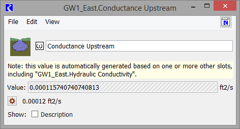 Screenshot of Scalar Slot dialog showing source slot functionality.
Screenshot of Scalar Slot dialog showing source slot functionality.Scalar Slots With Expression
This slot, similar to the Series Slot with Expression, is used to evaluate an expression that evaluates to only one value, i.e. timestep independent. See Series Slots With Expression for details on Series Slots with Expression, as that information is valid here too. The difference is that the scalar expression slot does not have an Evaluation Range, it will evaluate for the single value only. Like the series expression slot, the user can configure when it evaluates. Use the Expression, then Evaluation Time menu to choose.
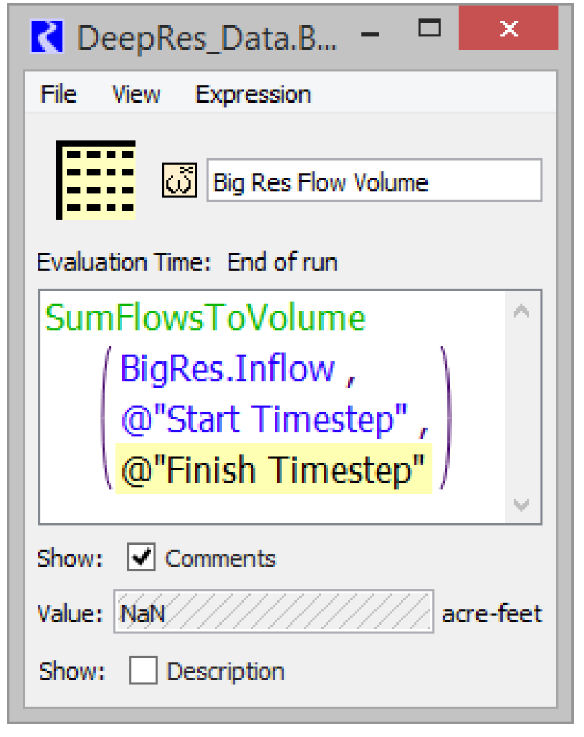
The Scalar Slow with Expression always opens in its own dialog box so you can see the expression. You can drag the scalar slot icon onto an existing Slot Viewer (Scalar) or use the File and then Dock in Slot Viewer menu.
Mass Balance Summary Slots
The Mass Balance Summary slot is a user-defined hierarchy of series slot collections used to check (i.e. sum) mass balance across many objects. The collections are themselves series slots representing the sum of the contained slots. These slots can be used within RPL expressions and any other place where series slots are used.
There are two levels of within a Mass Balance Summary slot:
• Water Balance. The sum of one or more Slot Sums. For example, a water balance might represent all water flowing in/out of the main channel or all flows in the groundwater.
• Slot Sum. The sum of one or more series slots. Slot sums are useful to summarize or classify different slots. For example, a Slot Sum might represent all the seepage, evaporation, diversions or return flow slots. The sum is represented as either the positive or negative sense. Negative Slot Sums are subtracted from their containing Water Balance. Positive Slot Sums are added in the containing Water Balance. Only flow/volume or mass (unit type) series slots having the model run timestep size can be used. References to RPL expression slots are supported for entities not represented by simulation slots.
Figure 5.31 shows the icons for the Mass Balance Summary Slot and the Computed Mass Balance Slots (i.e. Water Balances and Slot Sums).
Figure 5.31
The Computed Mass Balance Slots are computed:
• On demand (by you) and/or
• At the end of a run, immediately after the evaluation of post-run RPL expression slots.
Also, a list of RPL expression slots to be evaluated after a Mass Balance Summary slot computation can be specified within the summary definition. For example, this can be used for annualization of mass balance summary results.
The screenshot shows the dialog for a Mass Balance Summary Slot. Colors are associated with the three collection levels:
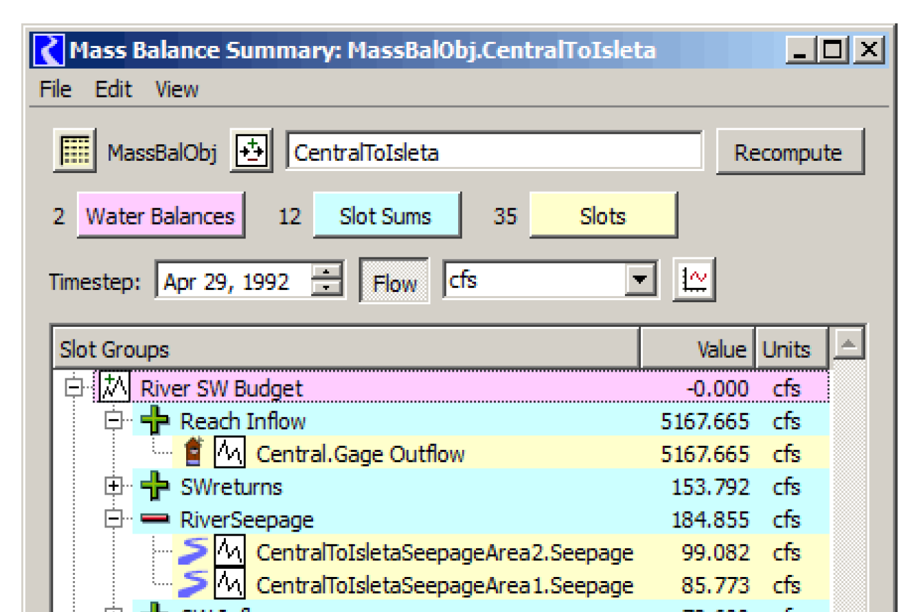
The color buttons at the top of this dialog function as a legend for the three levels. Also, selecting those buttons open the tree items in the list to the corresponding level. Also individual collection items can be opened and closed in the usual way, by selecting the tree controls.
Finally, the slots can be shown in any user units and plotted as needed.
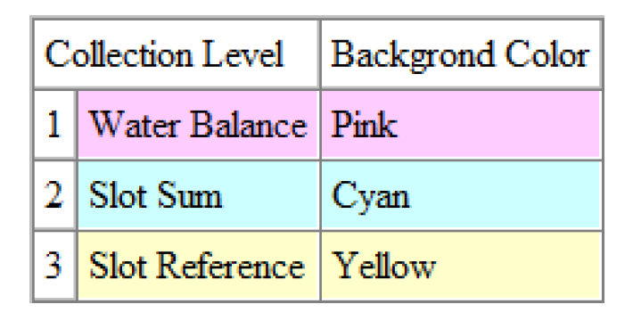
Creating a Mass Balance Summary Slot
A Mass Balance Summary Slot can be created by selecting the Add Mass Balance Summary operation.
The name of the new Mass Balance Slot can be edited in the dialog. When the entered name is not valid, the text in the name entry field is shown in red.
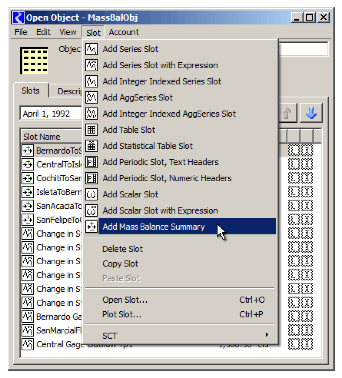
Configuring a Mass Balance Summary Slot
Editing the configuration of a Mass Balance Summary Slot can be enabled or disabled. It is initially enabled on a newly created slot. Editing can be enabled or disabled with the following controls:
• The lock icon toggle button in the bottom left of the dialog. 
• The Enable editing item in the right-click context menu.
• The Enable editing item in the Edit menu.
Right-clicking the list outside of any defined items (e.g. when the list is empty) shows a simple context menu including the Add Water Balance operation.
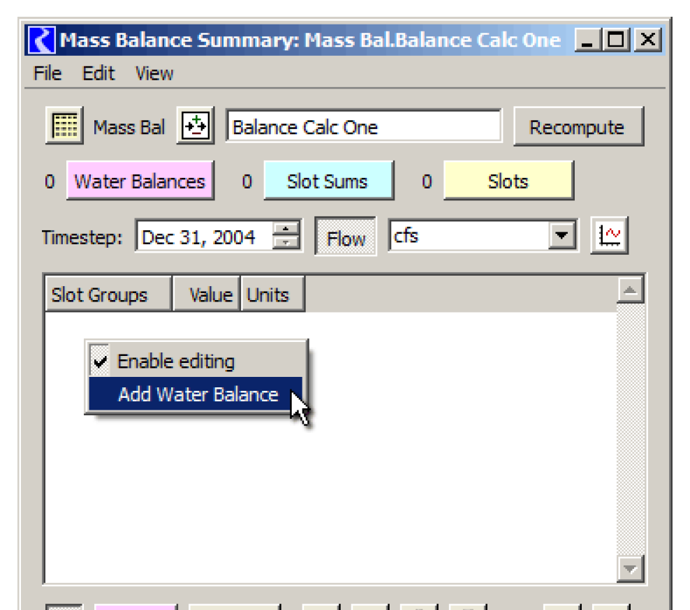
The buttons along the bottom of the dialog are also context sensitive; that is, their operation and enabledness depends on the selection within the slot list. When no items are selected, the New button also adds a water balance to the list.
When new Water Balances or Slot Sums are created, they are given a unique default name. The name can be edited inline by double-clicking the name.
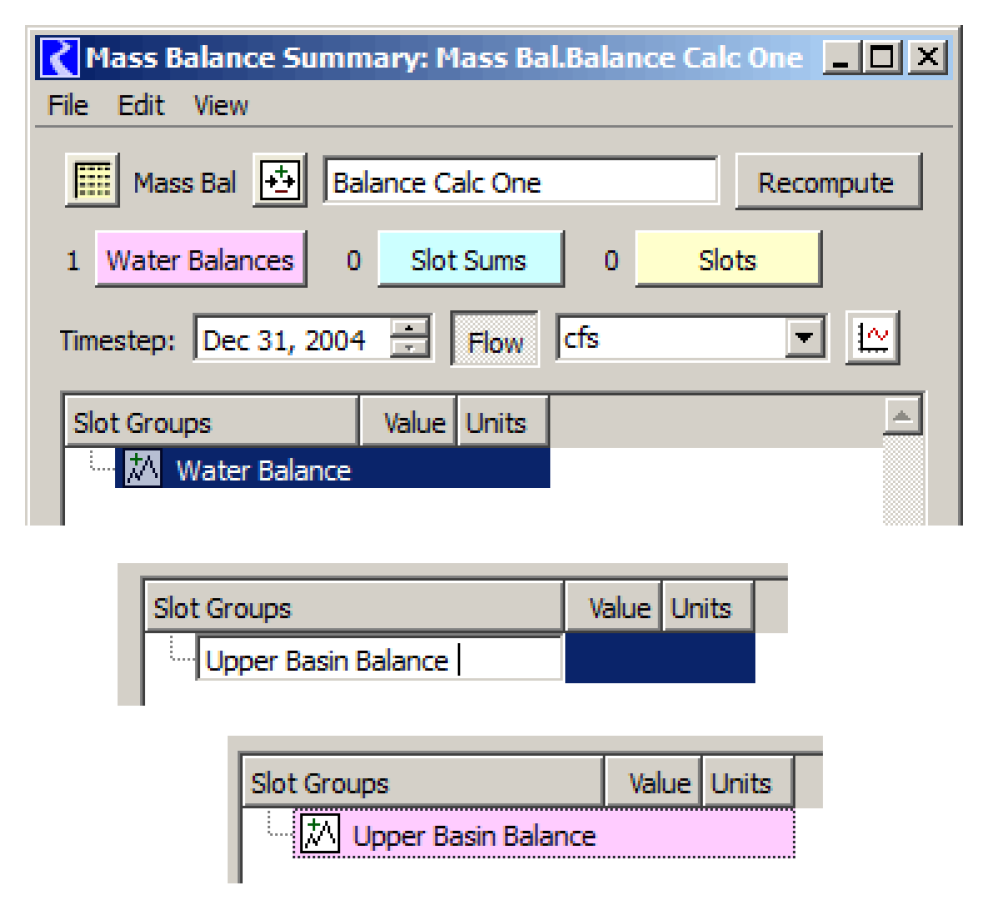
Slot Sums can be added to Water Balances, and Slot References can be added to Slot Sums using the Add context menu operation or the bottom context buttons.
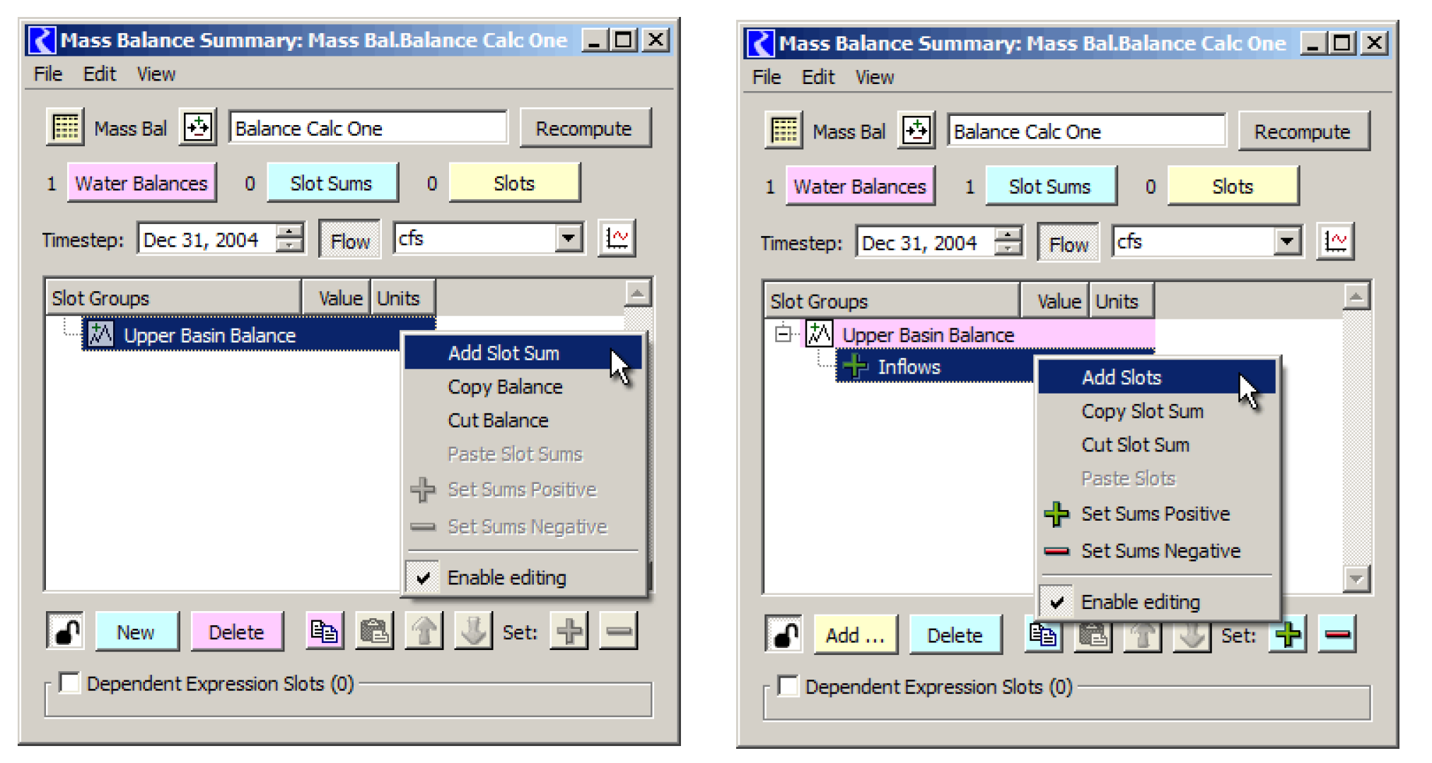
When adding Slots, the slot selector dialog is shown. This will allow the selection of only series slots. The slot selector’s unit type filter will be shown, initialized to “Flow”. It is also valid to select “Volume” slots which represent a non-static volume entity; that is, those that can be converted to “Flow” by dividing its value by the timestep interval (i.e. volume per time). (The computed results will be strange if a static volume slot, such as Reservoir Storage, is selected).
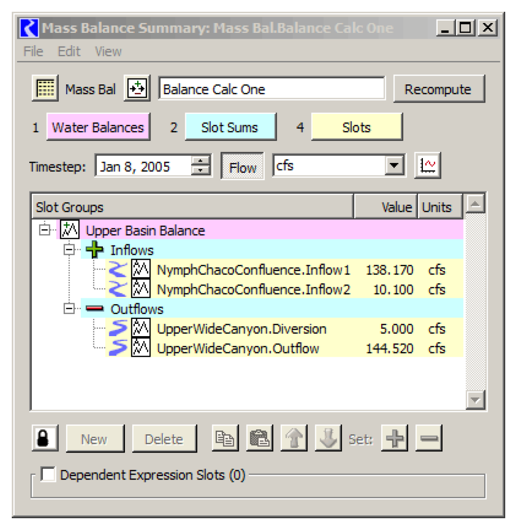
Alternatively, slots representing mass units (g, kg, tons, etc) can be chosen. This is particularly useful when looking at the salinity mass balance across many objects.
Note: A Mass Balance Summary can either show Flow/Volume units or Mass units, but not both. If both types of slots are shown (or slots with any other unit type), an error will be issued when the mass balance is computed.
Figure 5.32 shows the operations provided by the first several buttons, as a function of the selected item or items. Tooltips on these buttons provide additional information.
Figure 5.32
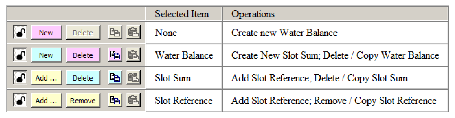
The New, Add, and Paste operations are enabled only for single-item selections. The Delete, Remove, and Copy operations are enabled on single or multiple selections when all selected items are at the same level. The enabledness of the Paste operation depends also on the type of items (Water Balances, Slot Sums, or Slot References) in the clipboard. You must confirm Delete / Remove operations.
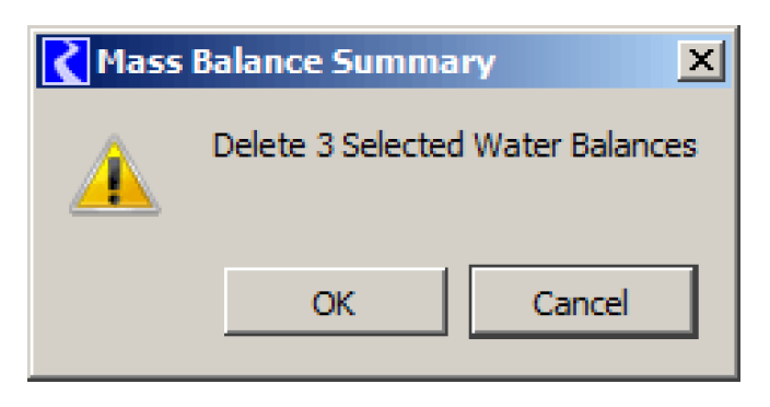
The Up and Down arrows move the selected items up or down within the set of “sibling” items. They are enabled only when the selected items are all at the same level.
The  and
and  buttons affect the Slot Sums within the set of selected items.
and buttons affect the Slot Sums within the set of selected items. Note: When the mass balance summary is computed, the values of positive Slot Sums are added to the containing Water Balance; the values of negative Slot Sums are subtracted.
RPL Expressions for Other Slots
For any value not provided as a RiverWare slot, you will need to define and refer to a RPL expression slot. Figure 5.33 is an example of the inclusion of a change in storage expression slot from the previous to the current timestep.
Figure 5.33
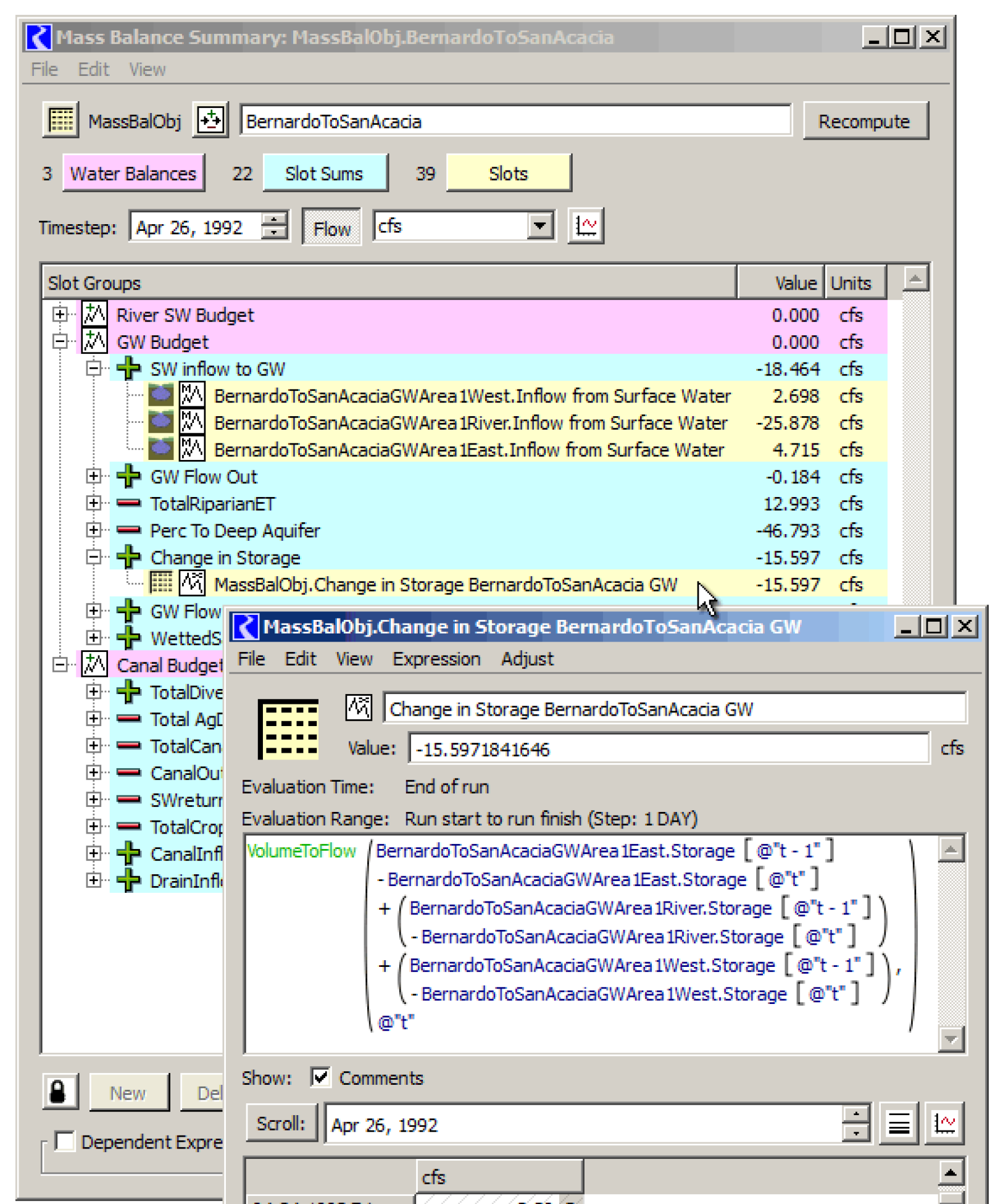
Display Operations
The Mass Balance Summary Slot dialog shows a single timestep value of all contained series slots.
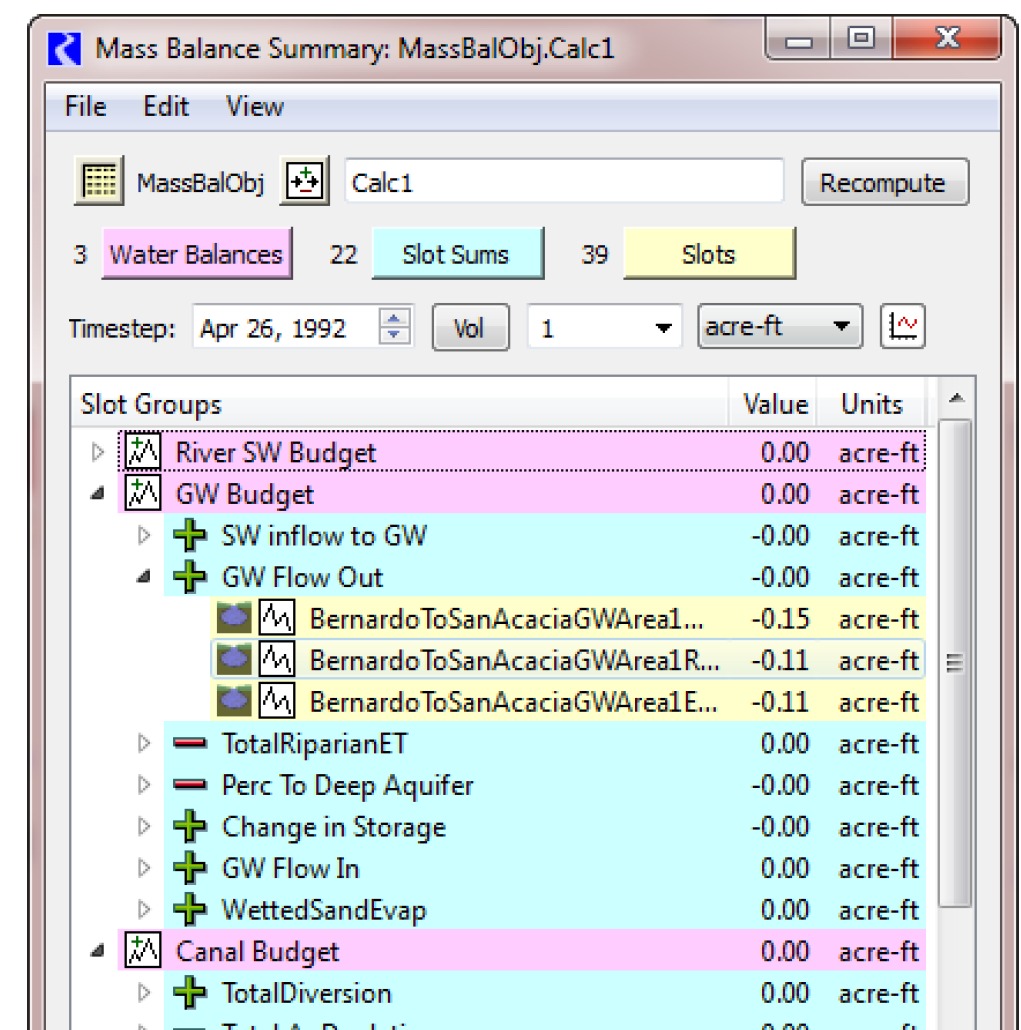
Note: All Water Balances, Slot Sums and series slot references must have the same timestep size as the model run. Water Balances and Slot Sums are computed for the model run interval (start to finish timesteps).
Units
In this dialog, series values have the following options:
• Flow or Volume units. Volume values are converted to flows by dividing by the timestep interval. The individual settings for Flow and for Volume units are separately retained. That is, selecting the Flow and Volume button switches between the last selected unit for those two unit types.
• Mass units. This is typically used for salinity.
Note: A Mass Balance Summary can either show Flow/Volume units or Mass units, but not both. If both types of slots are shown (or slots with any other unit type), an error will be issued when the mass balance is computed.
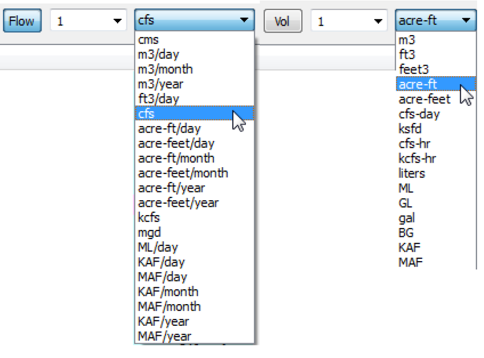
The selected unit type, scale and unit is both a display setting and a configuration setting; when the mass balance summary is computed, the computed slots are shown with these units. Precision can be set from the View, then Set Precision menu.
In fact, changing the unit, scale, or precision from this dialog actually changes the active Unit Scheme (by adding exceptions). You can also change the settings from the Unit Scheme Manager by changing attributes or activating a different scheme. See Unit Schemes for details.
Note: When the computed results (Water Balances and Slot Sums) are referred to by RPL expressions, the units must work correctly or an error will be issued. Unit type incompatibilities will be reported by the RPL expression evaluation mechanism in the usual way.
Tree Display
As previously mentioned, the level Legend buttons function to open the entire tree to the indicated level. Of course, individual tree items can be opened or closed by selecting the standard tree controls.
Figure 5.34
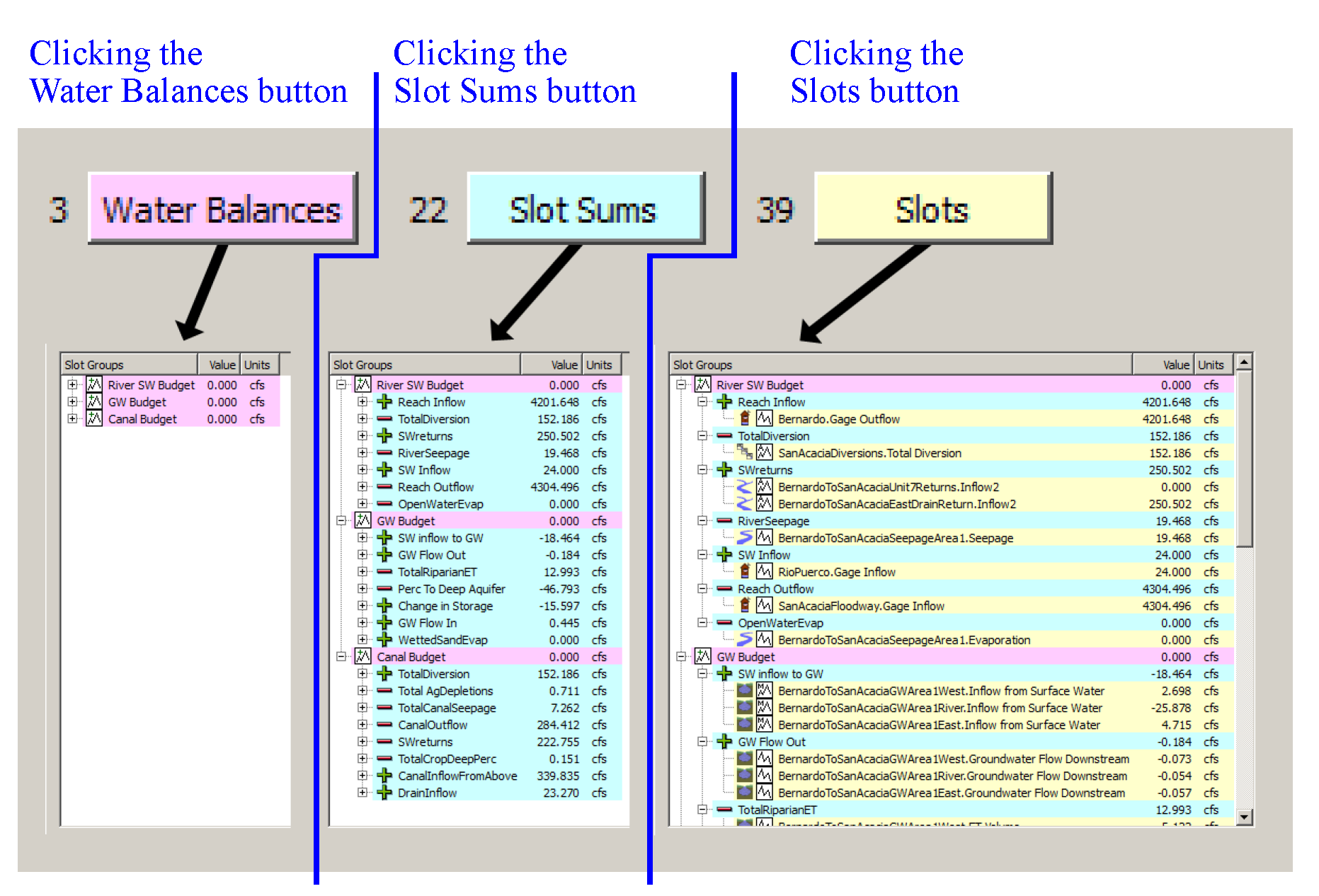
The View menu provides operations that affect data display within this dialog.
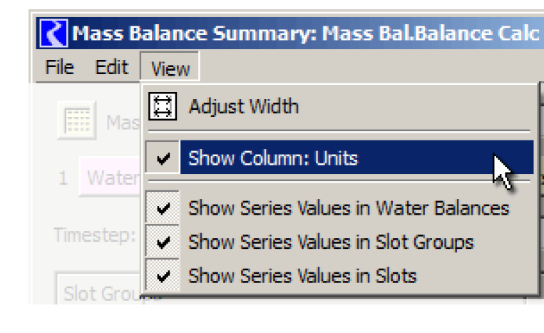
Show Column: Units
The units column in the slot list can be hidden. But, if slots having different unit types (other than flow/volume or mass) are added to the list, units are unconditionally shown and the option to hide the units column is disabled.
Show Values
You may want to hide values at any of the levels, so that only comparable values (at the same level) are displayed. The three Show Series Values toggles in the View menus are used to show or hide the numeric values; Figure 5.35 illustrates.
Figure 5.35
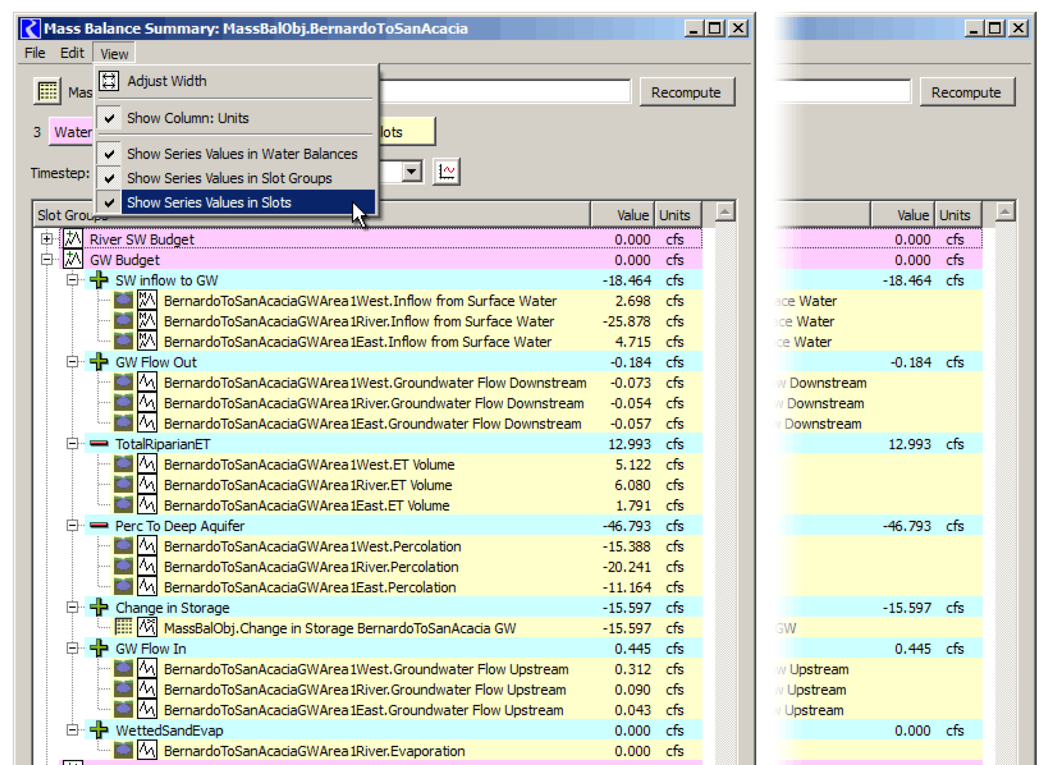
Other Display Operations
From the Open Mass Balance Summary Slot dialog, you can perform the following operations:
• Show selected slots in an open slot dialog.
• Show slots in a new SCT or in the single open SCT. You can show either the visible (in the tree), or only the selected slots.
• Plot the selected slots.
• Copy selected slots, e.g. to an Output Device or to the Snapshot Manager.
These options are described in the following sections.
Show Computed Slots in an Open Slot Dialog
As currently implemented, Water Balances are generated as aggregate series slots and each of the Water Balance’s Slot Sums are generated as series slot columns on that aggregate. Use the Open Slots context menu to show the slot dialog for the selected component (editing disabled).
Note: There is currently no indication of the Slot Sums’ “sense” being positive or negative.
Values are displayed with a crosshatch indicating that they are “read-only” (non-editable). In Figure 5.36, the not-quite-zero value in the “Value” line edit field from the single selected cell (upper left cell); this sort of value will be typical of actual computed Water Balance values (due to convergence). Enabling the display of the selection statistics (from the View menu) and selecting the first column provides a convenient way to determine whether or not the whole Water Balance series is zero.
Figure 5.36
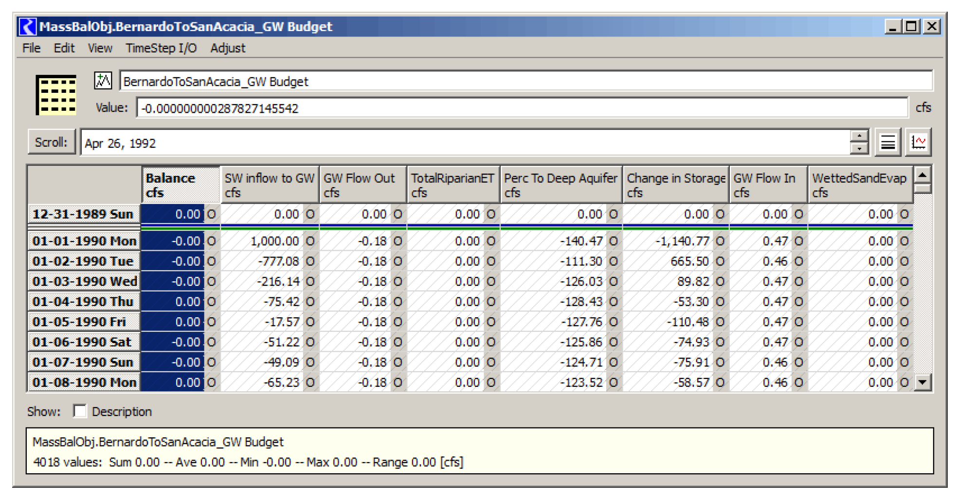
Show Slots in an SCT
Computed summary and referenced slots can be shown in an SCT. If a single SCT is open, slots from the Mass Balance Summary dialog can be added to that SCT (the SCT must have the same timestep size as the model run).
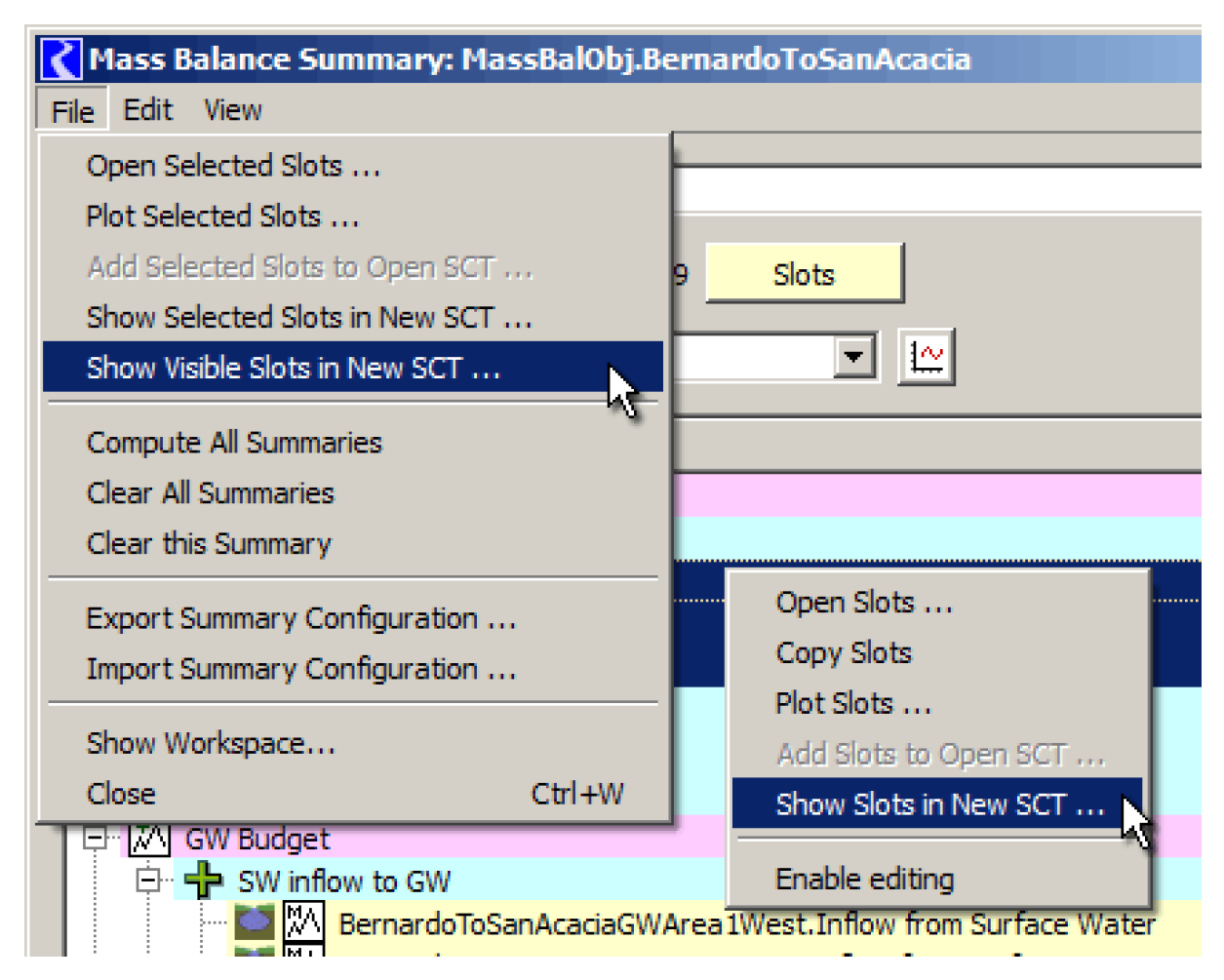
The File menu Show Visible Slots in New SCT option shows all slot items current visible in the slot list (i.e. excluding those hidden under a closed tree branch).
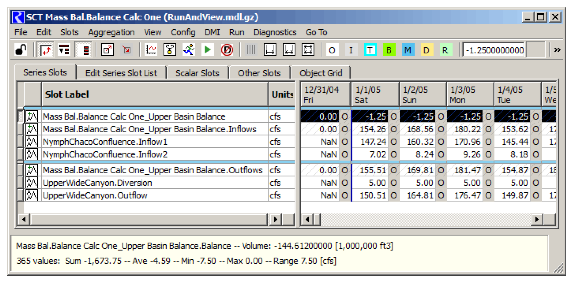
Note: Water Balance and Slot Sum slots are shown with the values and units set at the time of the most recent mass balance computation; that is, not necessarily the current unit setting in the Open Mass Balance Summary Slot dialog. If referenced slots are including in the “show in SCT” operation, they will be shown with their currently configured (or “active”) units. And if they are editable slots, they will be editable in the SCT. (Rows that are not cross-hatched can be edited directly.
Plot Slots
Computed summary and referenced slots can be plotted in a single plot. Those operations are visible in the menus shown in the prior section. The note above regarding the active units of computed and referenced slots applies also to Plots; that is, the units used will not necessarily be those of the current settings in the Open Mass Balance Summary slot dialog.
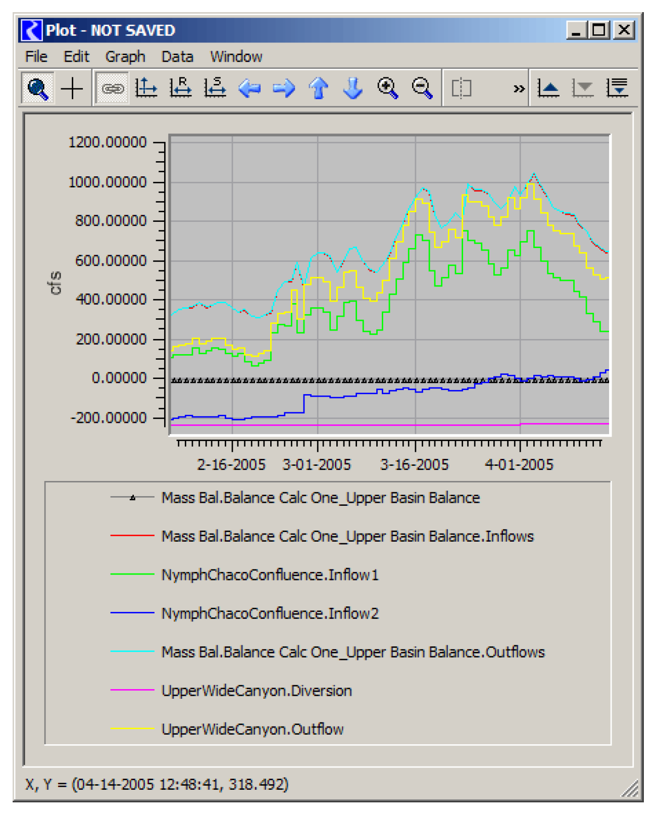
Note: All values are plotted in their positive (actual) sense; that is, values in negated Slot Sums are not shown as negated values.
Copy Slots
Computed summary and referenced slots can be copied to the RiverWare Slot Clipboard. From there, they can be pasted into various slot lists in RiverWare, including the general Output Device slot list and the Snapshot Manager slot list.
Examining the Mass Balance Summary Slot’s Series
The Mass Balance Summary Slot is itself a series slot and can be examined by selecting the Mass Balance Summary Slot icon button at the top of the dialog. (In a sense, a Mass Balance Summary Slot has two different open slot dialogs).
In Figure 5.37, all the values represented on the vertical axis are zero (to a precision of five fractional decimal digits).
Figure 5.37
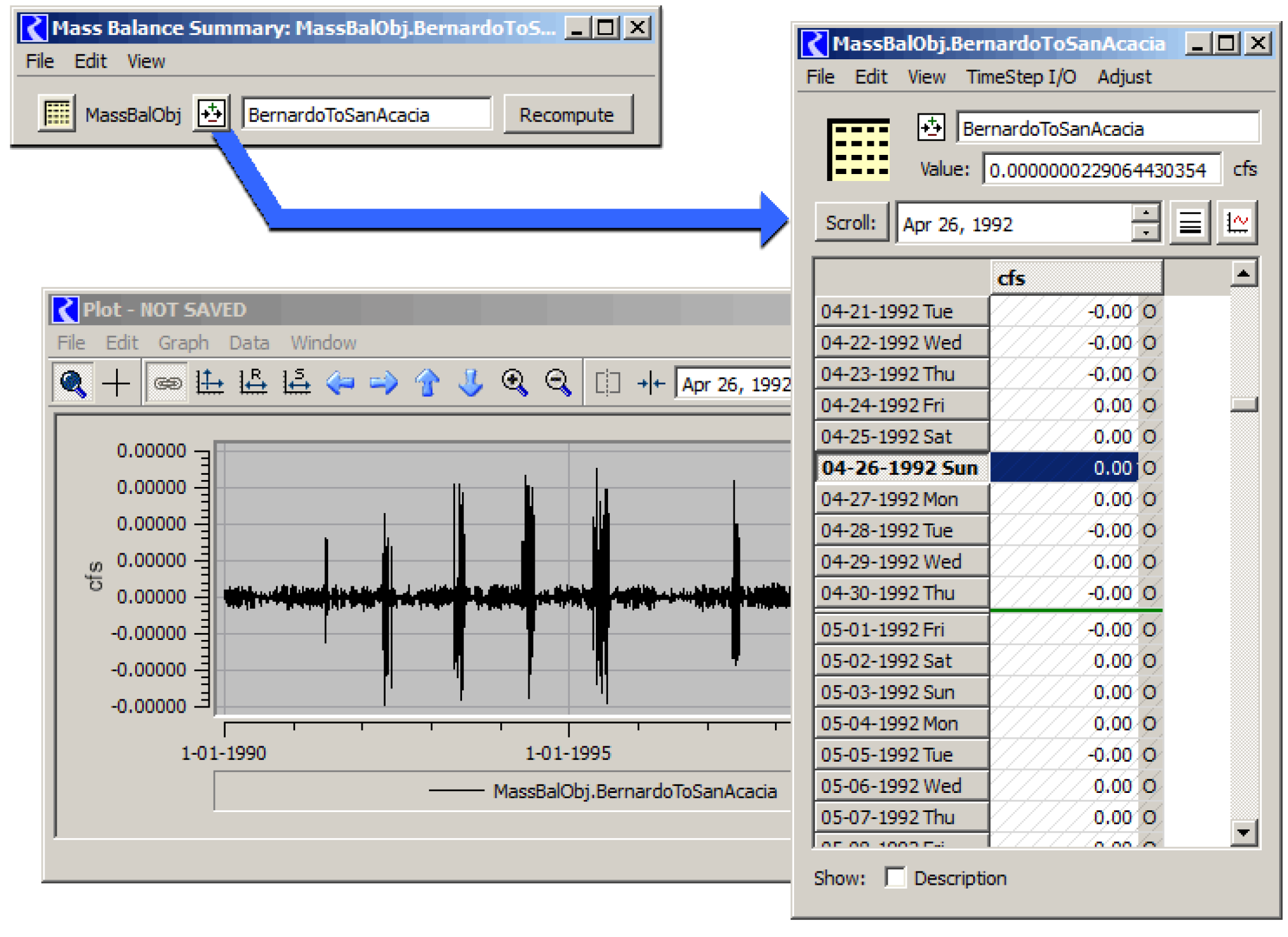
Dependent RPL Expression Slot Support
Mass Balance Summaries are designed in such a way that intermediate and final sum results (Slot Sums and Water Balances) are usable for custom user calculations implemented in RPL Expression Slots, such as annualization of values. In a run, the mass balance summary is computed after RPL Expression slots. To allow RPL expression slots to reference mass balance summary data, the Dependent Expression Slot List in a Mass Balance Summary is evaluated, in order, once, after each Mass Balance Summary is computed.
Dependent Expression Slot results will generally be incomplete when computing a Mass Balance Summary if the RPL Expression Slots in the list depends on sums from multiple mass balance summaries. The following provisions address this problem:
• The automatic end-of-run mass balance computations are performed in this order:
1. The RPL Expression slots in the Dependent Expression Slot Lists in ALL Mass Balance Summaries are cleared.
2. All Mass Balance Summaries are computed.
3. The RPL Expression slots in the Dependent Expression Slot Lists in ALL Mass Balance Summaries are evaluated.
• In addition, in the File menu, there is a Compute All Summaries option that perform this model-wide computation (the three steps in the prior item)
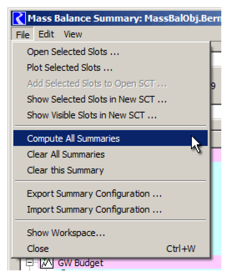
The Dependent Expression Slot panel at the bottom of the Open Mass Balance Summary Slot dialog implements editing and display operations similar to those of the main slot list.
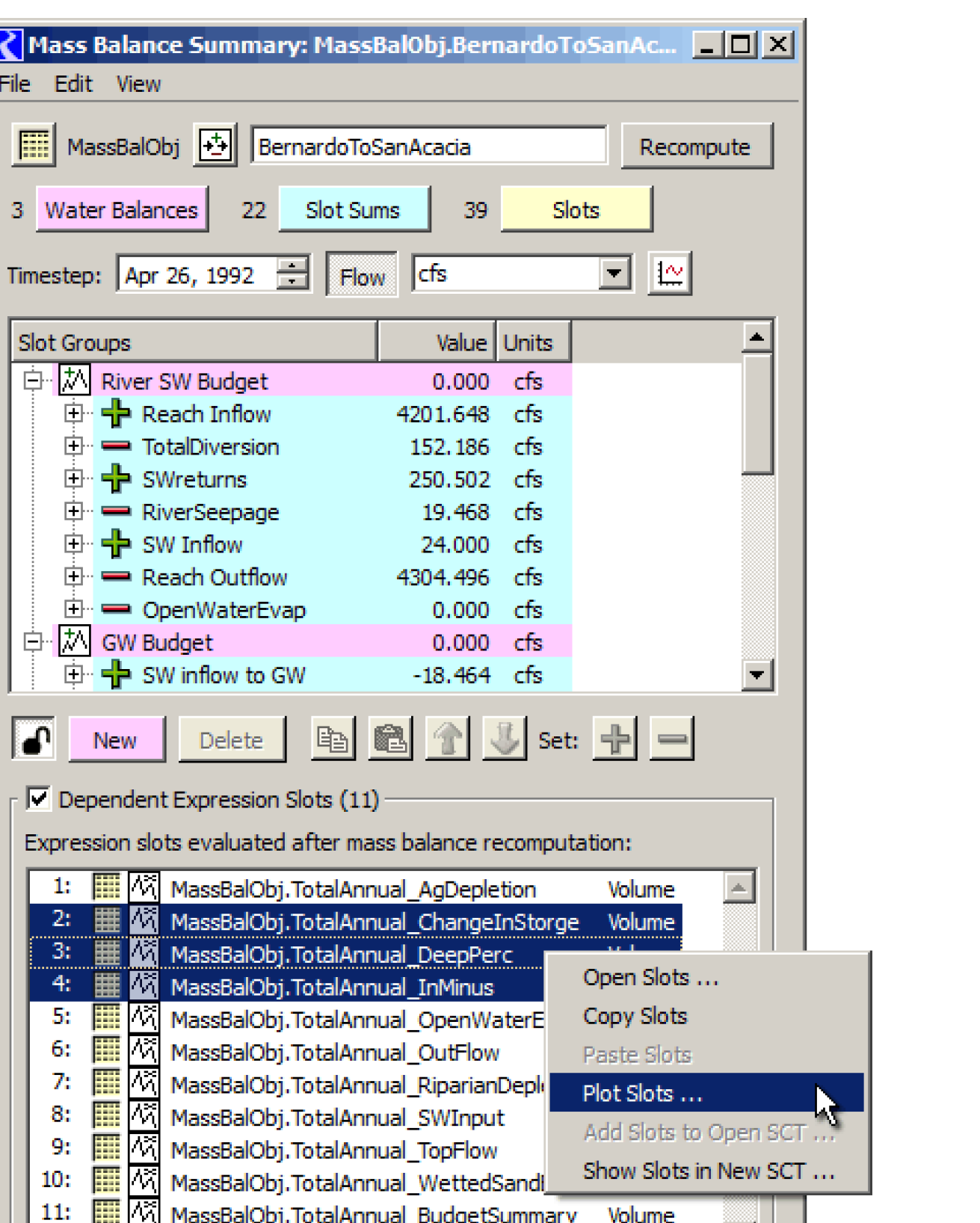
Note: If the dependent Expression Slots use a different from the model’s run timestep, they can’t be displayed in the same SCT as the computed summary slots and slot references.
Selecting the Add button opens the slot selector, initialized with Has RPL Expression and Unit Type (“Flow”) filters on by default.
Computation
When computed, the timestep size and timestep range of each of the Mass Balance Summary and Slot Sums are set to the step size and range of the run controller. The unit type and configured display units are set to those specified. For each timestep in the run time range, any of the contained slots having a valid value at that timestep contributes that value to the Slot Sum or Water Balance’s value at that timestep. NaNs are ignored (effectively zero). The computed slots are set to be “read-only”.
Limitations of the current Mass Balance Summary Computation:
• No “routed terms”. A timestep offset cannot be applied to any slot reference within a Slot Sum, or to any Slot Sum within a Water Balance.
• No knowledge of static volumes. The mechanism unconditionally converts all volumes to flows by dividing the volume by the timestep size (for each timestep). See RPL Expressions for Other Slots for a RPL implementation of the change in storage calculation.
Mass Balance Summary Computations are performed in these ways:
• By selecting Recompute in the Open Mass Balance Summary Slot dialog.
• By selecting Compute All Summaries in the File menu of that dialog.
• Automatically, at the end of a run, immediately after the end-of-run RPL Expression Slots evaluation. This is performed unconditionally.
As a tool for debugging and testing Mass Balance Summary implementations (including user definitions), operations to clear an individual Mass Balance Summary, and all Mass Balance Summaries (including Dependent Expression Slots) is provided in the File menu.
Persistence
All Mass Balance Summary configuration information is stored on the Mass Balance Summary Slot. This is applied both in the RiverWare model file and in Export files.
A Mass Balance Summary Slot’s computed slots are created as (effectively) invisible slots on the same object. They do show up in the slot selector!
A Mass Balance Summary Slot’s configuration can also be saved to, and read from a file using Export and Import operations in File menu.
Time Aggregation Series Slots
Time Aggregation Series Slots temporally aggregate another series slot. For example, you might aggregate a daily flow to an annual average. They can be recomputed manually or automatically at the end of a run. The configuration of a Time Aggregation Series Slot includes the following properties. Figure 5.38 illustrates.
Figure 5.38
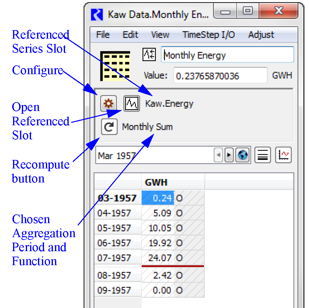
• The series slot to be aggregated, chosen using the slot selector.
• The aggregation function, one of:
– Sum. Add the values during the aggregation period.
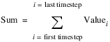
Note: For slots with a rate unit type (flow or velocity), a true sum does not make sense and is therefore not an option in the menu. Instead, use the average which represents a time weighted average. Change the display units as needed to see the values desired.
– Average. Report the mean during the aggregation period.
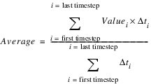
– Minimum. The smallest value (in units displayed) in the aggregation period is reported.
– Maximum. The largest value (in units displayed) in the aggregation period is reported.
– First value. The first value in the aggregation period is reported.
– Last value. The last value in the aggregation period is reported.
• Choice of aggregation period, as follows:
– 1 Hour
– 6 Hour
– 1 Day
– 1 Month
– 1 Year, Calendar Year
– 1 Year, Water Year*
• The Units you wish to show, including display unit, scale, precision, and format.
• If you wish to evaluate them at end of run.
• What to do when encountering NaN.
Functionality is provided to duplicate a Time Aggregation Series Slot for the same named slot on multiple other “similar” objects.
Configuration Settings
Once created (from the Object’s Slot, then Add Time Aggregation Series Slot menu), open the slot dialog to configure the slot. Configuration controls are available in a separate dialog which is shown by selecting the Configure icon  .
.
.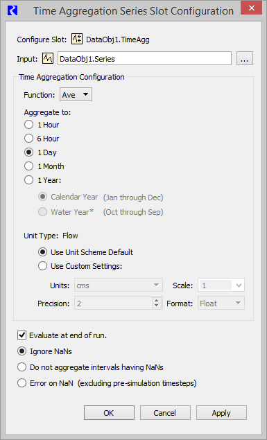
1. Select the slot to aggregate using the Input field.

2. Select the aggregation function; use the Function menu to select the aggregation function to be used. See Time Aggregation Series Slots for details on the functions.
3. Select one of the following the aggregation periods (only aggregation periods larger than the source slot’s timestep are available):
– 1 Hour
– 1 Day
– 6 Hour
– 1 Month
– 1 Year - Calendar Year
– 1 Year - Water Year*
4. Hover over the Water Year text to display a tooltip. See Annual Aggregation Support for Non-calendar Water Years for details on Water Year.
5. Then choose the Units to show for the aggregated data. The Unit Type is fixed to the Unit Type of the referenced series slot. But you can specify any display units to use. For example, you can show daily flows in cfs averaged as monthly values, displayed in acre-feet/month. The options are as follows:
– Use Unit Scheme Default. When this is selected, the unit scheme specification, including any slot name exceptions will be used. See Standard Units for details on Unit Schemes.
– Use Custom Settings. When selected, specify the units directly in this dialog.
Note: This will actually make a Slot Exception in the Unit Scheme with the specified units.
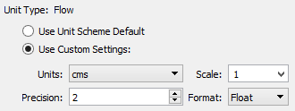
6. Optionally, enable automatic end of run evaluations. The Evaluate at end of run checkbox controls whether this slot is automatically evaluated (recalculated) at the end of the run. The end of run evaluations are performed after all end of run RPL Expression Slot evaluations. (So, it would be reasonable for a Time Series Aggregation Slot to aggregate an “end of run” RPL Expression Series Slot).
7. Select one of the following NaN value options:
– Ignore NaNs. NaNs do not contribute to the aggregated values. Intervals with some values and some NaNs will become values at the larger timestep.
– Do not aggregate intervals having NaNs. Any interval with NaNs are not aggregated. Intervals with some values and some NaNs will be NaN at the larger timestep.
Note: For the First and Last aggregation function, only the First and Last timestep is considered. Other timesteps do not matter in their NaN status.
– Error on NaN (excluding pre-simulation timesteps). An error is issued to diagnostics.
Annual Aggregation Support for Non-calendar Water Years
One of the supported aggregation modes is aggregation to Water Years, starting in a user-specified month.
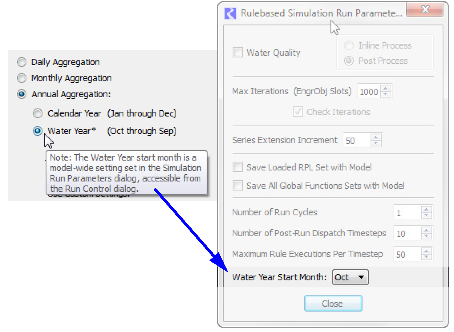
The Water Year Start Month is a model-wide setting, configured in the Simulation Run Parameters dialog, accessible from the Run Control Dialog; see Simulation Run Parameters for details.
Note: The resulting series with a 1 Year timestep is still nominally identified as a calendar year (ending on December 31). Water years are named by the year in which the water year ends, i.e. a water year from October 2000 through September 2001 is the “2001” water year.
Creating Similar Time Aggregation Series Slots for Different Objects
In a single operation, you can create a Time Aggregation Series Slot for the aggregation of the same series slot on multiple other selected simulation objects. For example, if a given time aggregation slot is annually summing the Energy slot on a power reservoir, similar aggregation slots can be created for all other power reservoirs, in a single operation. Figure 5.39 shows an example.
When a properly configured Time Aggregation Series Slot item is selected within an Object’s slot list, the Create Similar Slot for Different Objects operation under the Slot menu is enabled. Activating that menu item brings up the simulation object selector dialog where multiple objects can be selected. The selector is initialized to show objects of the same type as the object containing the reference slot (e.g. in this example, Power Reservoirs). Ultimately though, you can select a broader range of simulation objects.
The names of the new slots are devised as follows: If the originally selected time aggregation slot's name contains the name of the referenced slot's containing object, then the new names are that name, with the original containing object name replaced by the new selected objects. In the example, the original time aggregation slot named “Monthly Energy” is aggregating the “Kaw.Energy” slot. However, the originally selected time aggregation slot's name does not contain the name of the referenced slot's containing object, no direct name substitution is possible. Instead, the names of the new selected objects are appended to the slot name for the new slots: Monthly Energy_Eufaula, Monthly Energy_Hudson, and so forth.
Figure 5.39
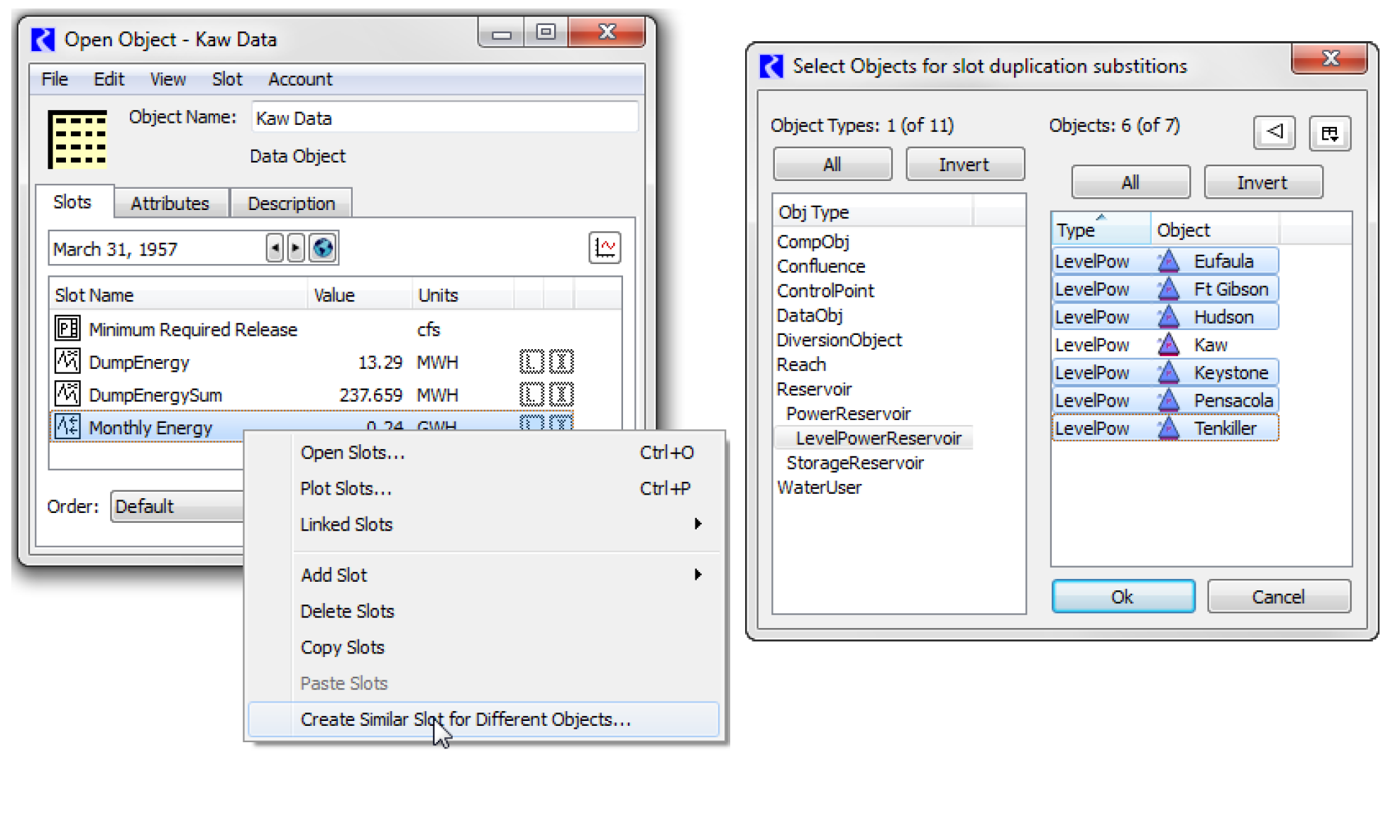
Time Disaggregation Series Slots
Time Disaggregation Series Slots temporally disaggregate another series slot into a smaller timestep. For example, you might disaggregate a daily flow to an hourly flow using the same value for each hour in the day. They can be recomputed manually or automatically at the end of a run. The configuration of a Time Disaggregation Series Slot includes the following properties. Figure 5.40 illustrates.
Figure 5.40 Screenshot of Time Disaggregation Series Slot
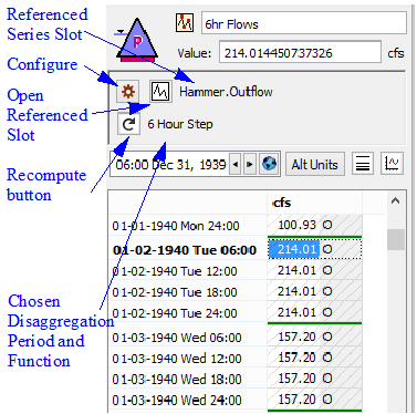
• The series slot to be disaggregated, chosen using the slot selector.
• The aggregation function, one of:
– Step. Use the value at the end of the larger timestep for each value in the smaller disaggregated timestep. This is useful when you need the average over the period to remain the same, for example for FLOW values.
– Interp. Linearly interpolate between the values on the larger timestep. This is useful when the values change linearly over the disaggregation period. For example, Pool Elevations can be assumed to change linearly from one larger timestep to another.
• Choice of disaggregation period, as follows:
– 1 Hour
– 1 Day
• The Units you wish to show, including display unit, scale, precision, and format.
• If you wish to evaluate this slot at end of run.
• What to do when encountering NaNs.
Functionality is provided to duplicate a Time Disaggregation Series Slot for the same named slot on multiple other “similar” objects as described in Creating Similar Time Disaggregation Series Slots for Different Objects.
Configuration Settings
Once created (from the Object’s Slot, then Add Time Disaggregation Series Slot menu), open the slot dialog to configure the slot. Configuration controls are available in a separate dialog which is shown by selecting the Configure icon .
.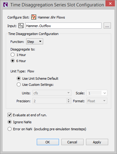
1. Select the slot to disaggregate using the Input field.
2. Select the disaggregation function; use the Function control to select the aggregation function to be used. See Time Disaggregation Series Slots for details on the functions.
3. Select one of the following the disaggregation periods (only disaggregation periods smaller than the source slot’s timestep are available):
– 1 Hour
– 1 Day
4. Then choose the Units to show for the disaggregated data. The Unit Type is fixed to the Unit Type of the referenced series slot. But you can specify any display units to use. The options are as follows:
– Use Unit Scheme Default. When this is selected, the unit scheme specification, including any slot name exceptions will be used. See Standard Units for details on Unit Schemes.
– Use Custom Settings. When selected, specify the units directly in this dialog.
Note: This will actually make a Slot Exception in the Unit Scheme with the specified units.
5. Optionally, enable automatic end of run evaluations. The Evaluate at end of run checkbox controls whether this slot is automatically evaluated (recalculated) at the end of the run. The end of run evaluations are performed after all end of run RPL Expression Slot evaluations. (So, it would be reasonable for a Time Series Disaggregation Slot to disaggregate an “end of run” RPL Expression Series Slot).
6. Select one of the following NaN value options:
– Ignore NaNs. NaNs do not contribute to the disaggregated values. Timesteps with NaN values will remain NaNs at the smaller timestep.
– Error on NaN (excluding pre-simulation timesteps). An error is issued to diagnostics if a NaN is found.
Creating Similar Time Disaggregation Series Slots for Different Objects
In a single operation, you can create a Time Disaggregation Series Slot for the disaggregation of the same series slot on multiple other selected simulation objects. For example, if a given time disaggregation slot is disaggregating the Pool Elevation slot on a power reservoir, similar disaggregation slots can be created for all other power reservoirs, in a single operation. This operation is identical to creating similar time aggregation slots for different objects. See Creating Similar Time Aggregation Series Slots for Different Objects for more information.
List Slots
A List Slot is used to store a collection of non-numeric data, typically a group of objects. Figure 5.41 shows a sample Upstream Reservoirs List Slot.
Figure 5.41
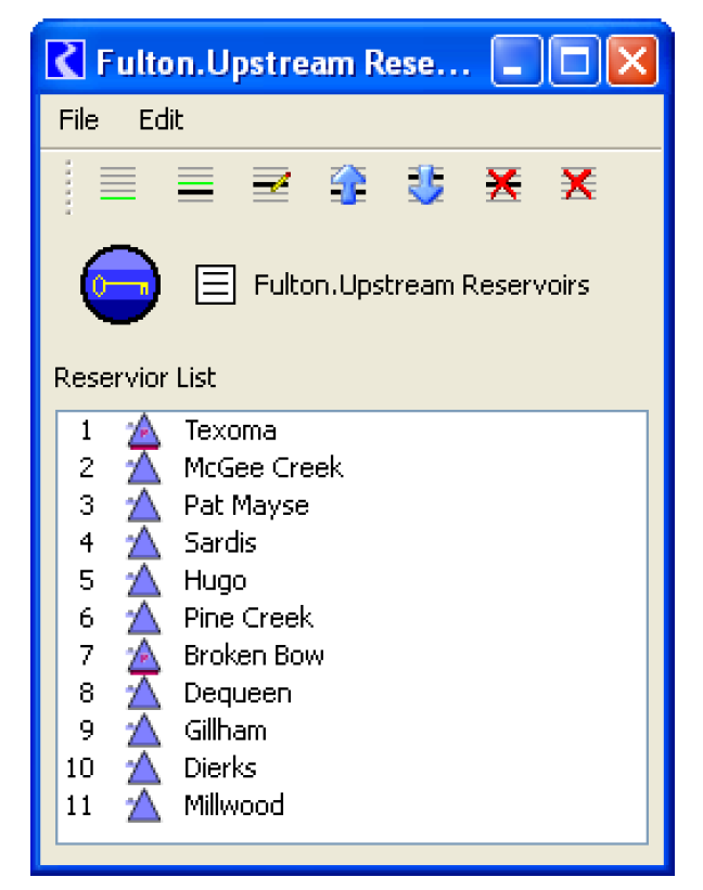
This slot contains the Reservoirs that are upstream of the given control point. It is used in the Regulation Discharge and Flood Control algorithm to specify the reservoir which contribute to the flow at this control point. Figure 5.42 shows the options available from the Edit menu, from the toolbar icons, and from the right-click context menu:
Figure 5.42
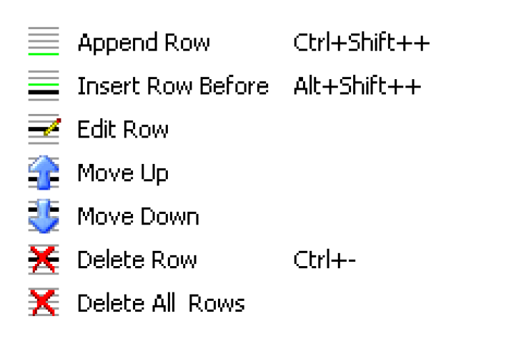
On a List Slot that contains either Objects, Slots, Accounts, or Supplies, when the user selects either Append Row, Insert Row Before, or Edit Row, a selector will open allowing the user to choose the appropriate items.
Revised: 08/02/2021