
Release Notes Version 1.0
RiverWare is a new river basin modeling software tool which can load and run models built with PRSYM. This document describes new features, enhancements and changes that are included in RiverWare Version 1.0, released on May 7, 1997.
These changes are new to the executable since the release of PRSYM Version 3.1 on July 29, 1996.
Direct questions to CADSWES Technical Support at (303) 492-0908 or e-mail: usersupport@cadswes.colorado.edu
Required Model File Updates
Aggregate Diversion Site and Water User slot name changes
Many slots on Aggregate Diversion Site and Water User Objects have been renamed. In order to preserve the data in Aggregate Diversions of existing models, a conversion script, included with this release, must be run. The Perl language script is called modelConvert1.0, which is executed by typing the script name followed by the file name to be converted. Until the script is run or the model file is saved under the new executable, a confirmation window will be generated at load time warning that conversion may be necessary. For more details on this procedure, see“Renaming of Slots”.
Special Attention Notes
Name Enforcement
Names of objects, slots, and DMIs are now limited to lowercase and capital letters, spaces, and underscores. Existing models which contain illegal characters in object and/or slot names will have these characters automatically converted to a legal text representation when the model is loaded. Expression slots, DMIs, and rules, however, will not automatically be updated to reflect the new names. Explicit updating of these references may be necessary.
solveMB_givenEnergyInflow dispatch method
A bug which prevented Level Power Reservoirs dispatching given Energy and Inflow from iterating to a proper Outflow has been fixed. Reservoirs dispatching under this dispatch method may also have incorrectly mass balanced. Differences in solutions should be expected between RiverWare Version 1.0 and versions of PRSYM when models contain any Reservoirs dispatching under this condition.
Known Bugs and Workarounds
Locator View Refresh
The Locator View, described in detail below, does not properly refresh the view of the workspace outside of the highlighted rectangle when objects or links are rearranged on the workspace with the Locator View dialog open. The dialog may be forced to refresh by closing and then re-opening it.
SCT Menu Bar
The menus at the top of the SCT can be made to “freeze” through a specific series of steps. This results in the menus’ sub-items not being displayed when the heading is selected. This situation will only occur if a run is initiated by dragging from the Run menu down to Start Run... before releasing the mouse and highlighting a cell during the run. When model execution ends, the menus will be frozen. To restore the use of the menus, select any heading and drag the mouse laterally to another heading. This is a GUI environment bug and may not manifest itself with all X window systems.
Confirmation Dialogs Running Open Windows
Running RiverWare under the Open Look environment causes several GUI peculiarities. The most notable problem is that confirmation dialogs are generated with only one option, the Yes button. In order for the GUI to behave similarly to XWindows, Galaxy users should launch the executable with an OpenLook “look and feel” command line argument:
% RiverWaret -laf ol
Model Loading and Saving
Name Enforcement
Names of objects and slots are now limited to lowercase letters (a through z), capital letters (A through Z), spaces ( ), and underscores (_). Models previously built under versions of PRSYM may contain illegal characters in their slot or object names. These characters are now converted to legal text representations during model loading. A List Notice window is generated to indicate the illegal names detected.
The converted names are displayed in the Diagnostics Output Window next to the old names. The RiverWare assigned names may be changed to any other legal name once the model is loaded. Renaming automatically updates expression slots, but will not update constraints, DMIs, or rules. A regular expression search-and-replace is recommended to easily update external files. Illegal characters are converted to the character name surrounded by underscores as below:
! | converts to | _exclamation_ | @ | converts to | _at_sign_ |
# | converts to | _pound_sign_ | $ | converts to | _dollar_sign_ |
% | converts to | _percent_ | ^ | converts to | _carrot_ |
& | converts to | _ampersand_ | * | converts to | _asterisk_ |
( | converts to | _left_parenthesis_ | ) | converts to | _right_parenthesis_ |
- | converts to | _dash_ | + | converts to | _plus_ |
= | converts to | _equal_ | | | converts to | _pipe_ |
\ | converts to | _backslash_ | ~ | converts to | _tilde_ |
{ | converts to | _left_bracket_ | } | converts to | _right_bracket_ |
[ | converts to | _left_square_bracket_ | ] | converts to | _right_square_bracket_ |
: | converts to | _colon_ | ; | converts to | _semicolon_ |
< | converts to | _left_arrow_ | > | converts to | _right_arrow_ |
, | converts to | _comma_ | . | converts to | _dot_ |
? | converts to | _question_mark_ | / | converts to | _slash_ |
Quick Saving
The Model Save command now saves the workspace over the currently loaded file without invoking a file chooser. Output values are saved with the model by default. To save the model under a different name, or to prevent output values from being included in the model file, select Model Save As..., and follow the Saving procedure as in previous versions of PRSYM. The last Save As... parameters are then used for all subsequent Save commands. This new behavior is consistent with other standard software packages, but may confuse long-time users of PRSYM. It is recommended to write-protect important model files to protect them from accidental loss.
Summary Info
A new Summary Info... command is available from the Model menu in the main RiverWare workspace window. The command generates slot instantiation diagnostics and memory usage statistics in the Diagnostics Output Window. The messages provide information on the number and visibility status of instantiated slots as well as the number of slot proxies for each object on the workspace. Summary Info also provides total model memory usage statistics for each type of slot, including their total number and the memory required for an empty slot.
Simulation
Table Interpolation
Failed table interpolations now abort the simulation run in addition to producing a diagnostic warning message. Previously, table interpolation errors allowed the run to continue, often causing fatal errors later in the simulation. A diagnostic warning message provides the interpolation lookup value, the table column at which the lookup failed, the data range of this column, and the row number where missing data was expected.
Read Only Slots
Values in Data Object slots marked Read Only are no longer cleared at the beginning of a run. Previously, values at timesteps flagged as OUTPUT were automatically reset to NaN. In order to preserve values which may be needed for future scenarios, slots marked as Read Only no longer have their outputs cleared.
Invalid Timesteps
RiverWare now aborts a simulation with an error when an attempt is made to write a value to an invalid timestep. This occurred most commonly in the Thermal Object’s Adjusted Load slot. The Thermal Object calculations write data to this slot at hourly intervals regardless of the model run timestep. This bug has been fixed, but there may be other instances where an attempt is made to write a value to an invalid timestep. When such an attempt is made, RiverWare will now abort simulation with the message “Failed to set value to: value because the date is not contained within the time series.” This error may be prevented by setting a single input value in the erroneous slot at the initial timestep. The input value will ensure that the user-configured timeseries is not reset to match the run control during run initialization.
Run Control
Date Range
The range of allowable timeseries dates has been expanded to include all years between 1800 and 2300 A.D. All simulation calculations and/or value assignments performed within this range are valid.
Yearly Timestep
The Yearly timestep has been enabled as a valid simulation timestep. This step may be selected in the Run Control and slot Time Series Range dialogs.
Setting Run Times
The results of changing run times in the Run Control dialog have been updated to be more consistent. A change to the Initial, Finish, or Duration parameter now affects the run times as follows:
• A change to the Initial time modifies the Finish time accordingly. Duration remains the same.
• A change to the Finish time modifies the Duration accordingly. Initial time remains the same.
• A change to the Duration modifies the Finish time accordingly. Initial time remains the same.
Control Buttons
The behavior of the Run Control buttons has been revised. The Start button is no longer active during a paused run, and the Start and Step buttons now execute from the initial timestep when a run is stopped. The current behavior of all of the buttons is:
• Start: Execute a run from the initial timestep.
• Step: Execute the next timestep only. (If no run is in progress or a run is stopped, execute the first timestep.)
• Pause: Interrupt execution after the current timestep.
• Continue: Resume execution from the current timestep.
• Stop: Abort execution after the current timestep.
Loading State
The Simulation Run Status window has been expanded to include the execution state Loading. This state is displayed if the Run Status window is open while a model is loading. Once the model has completed loading, the status reverts to Loaded.
Stop During Initialization
A run may now be stopped during the initialization timestep. Previously, the Stop command would only be processed at the end of the timestep. In large models, this initialization could often take a significant amount of time to execute. The Stop command now intervenes to abort the run during this timestep.
Engineering Objects
Reservoirs: Modifications were made as follows
Beginning of Target Operation
The Target Operation code was rewritten to include a flag marking the Beginning of Target. A user-defined Beginning of Target timestep is marked with a TB, or Target Begin, flag in the Storage or Pool Elevation Edit Slot dialog. When solving a target operation, RiverWare searches backwards from the Target time until it finds a valid Target Begin flag. The Target Operation is solved using the value from the timestep prior to the Target Begin flag as an initial condition. If the timestep prior to the Target Begin does not have a valid Storage or Pool Elevation, or a valid input value exists between the Target Begin and the Target, the simulation aborts with an error. Likewise, if the Target Begin or Target timestep is already determined, simulation aborts. If no Target Begin flag is specified, RiverWare searches backwards to the first valid value and solves the Target Operation with this initial condition.
When a beginning of target is assumed in this manner, RiverWare marks the timestep where the Target Operation actually begins with a tb (lowercase) flag in the Open Slot dialog. This flag is treated as an output, and is automatically cleared at the start of the next run. Setting a Target Operation from an SCT generates both the Target and Target Begin flags, and clears any previous Target Operations which overlapped with the new range.
Figure 36.1 Prior to Target Operation
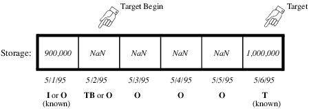
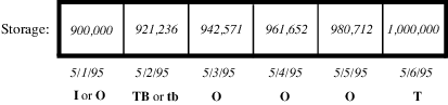
Figure 36.2 After Target Operation
Models previously built under PRSYM do not have Target Begin flags. These models will solve as they did before. RiverWare searches backwards until it finds a valid value and assumes a Beginning of Target time immediately after the valid value. In certain cases, however, models may have previously been overdetermined. Some older models may be overwriting Inflows or Outflows set by a Target Operation earlier in the run. This is caused by the Target Operation searching backwards too far for a beginning of target value which is not yet known. Due to dispatching order and other Target Operations, new Inflows or Outflows may be calculated which invalidate the original Target Operation. These modeling errors will now produce a “Setting Slot from multiple sources” message and abort simulation. The Target Operation may be corrected by explicitly setting a Target Begin flag at a timestep following the overdetermination.
Target Operation Calculation Category
The TargetOperationCalculationCategory has been expanded to all Reservoir objects. This Category was previously available only on Power Reservoirs. The noTargetCalc Method, which performs no calculations, has also been added to the two existing Methods and is now the default Method for this Category. Setting a Target Operation with the noTargetCalc Method selected will produce an error and abort simulation.
Hydrologic Inflows
A new User Method called noHydrologicInflow has been added to all Reservoirs. This is now the default Method for the HydrologicInflowCalculationCategory. This Method is used to model Reservoirs without the influence of hydrologic inflows, instantiates no slots, and requires no data.
The solveHydrologicInflow Method is no longer available on SlopePowerReservoirs and PumpedStorageReservoirs. Although the Method was previously selectable, it would not solve for timesteps where Hydrologic Inflow was not given on these Reservoirs.
The inputHydrologicInflow User Method has been modified not to initialize any linked slots at the Beginning of Run. The method previously initialized any unspecified Hydrologic Inflows and Hydrologic Inflow Adjust values to zero, and calculated the Hydrologic Inflow Net. It now checks that these slots are not linked prior to making any assignments. This allows values to propagate from other objects before dispatching.
Sediment Calculation
A new User Method Category called Sediment Calculation has been added to all Reservoirs. The Category is used to enable algorithms which adjust reservoir Elevation Volume and Elevation Area relationships in response to sediment inflow. There are two Methods available for selection within this Category, the default No Sediment Calc and CRSS Sediment Calc. The default Method performs no computations. Models previously saved under PRSYM will produce identical results when the default No Sediment Calc Method is selected.
The CRSS Sediment Calc Method is a reservoir sediment distribution algorithm based on the US Bureau of Reclamation’s Empirical Area Reduction Method. Sediment distribution is calculated by an iterative loop in which a total volume loss is derived from an assumed top of sediment elevation. The volume loss and top of sediment elevation are recalculated at each iteration, until the volume loss is equal to the given sediment inflow. The loss at each iteration is determined by an algorithm which utilizes elevation/area and elevation/volume data for the reservoir in conjunction with an empirical equation. This equation requires user-specified parameters to indicate the portion of total area which is taken up by sediment at any given elevation. The equation dictates the shape of the accumulated sediment and has a close relationship to the elevation-volume and elevation-area characteristics of the reservoir. The new elevation/area and elevation/volume data is stored in a polynomial coefficient table. This table is recalculated after each timestep. The actual Elevation-Area and Elevation-Volume tables used by RiverWare are adjusted following convergence of the solution, but prior to the hydrologic simulation.
The CRSS Sediment Calc Method is modeled after sedimentation calculations performed by the US Bureau of Reclamation’s Colorado River Simulation System (CRSS) model. The Method is initialized during TIMESTEPBEGINRUN. The User Input Elev Area Data is used to create the initial Elevation Volume and Elevation Area Tables which are required by the simulation. The elevation increments at which the two tables’ values are generated are determined by the Elevation Vol_Area Table Increment slot value. The Method initialization also uses the User Input Elev Area Data to create the Elevation Area Table Used and Elevation Volume Table Used. These tables are used solely for recalculating sediment distribution in later timesteps. The elevation increments for these tables are equal to those of the User Input Elev Area Table. Variable table increments allow sedimentation parameters to be calculated with a different precision than that used for the general Elevation Area and Elevation Volume Tables.
Input data is critically important for this Method. The close relationship between the empirical area reduction equation and the shape of the reservoir (reflected in the elevAreaTableInput table) makes this Method very sensitive to input data. The physical characteristics of the given reservoir must be considered when choosing empirical parameters for this Method. The Bureau of Reclamation currently considers four types of reservoirs, each having a corresponding set of empirical area reduction parameters. The reservoir type classification is based on shape, the manner in which the reservoir is to be operated, and the size of the sediment particles to be deposited, with the primary emphasis on shape. Tables are used to classify the reservoirs based on these characteristics. Once the type has been established, the parameter values for that type can also be taken from tables in the literature. An incorrect set of parameters for a given reservoir will lead to an inability to achieve convergence on the sediment distribution.
It is also important to note that this Method does not recalculate Elevation Area or Elevation Volume Tables during time horizon dispatching such as Target Operations. Models which do not solve chronologically may produce errors due to incorrect Elevation Area and Elevation Volume Tables. Contact CASDWES staff for additional information before implementing this new Method.
Following is a list of slots relevant to this method, which includes the slot name in bold type, the (slot) as it appears in the code in parentheses, the slot type (Multislot, etc.), the unit type(s) in all caps (LENGTH, FLOW, etc.), a brief description of the slot in italics, and additional comments in plain type.
Slots with Required Input Data
• Sediment Inflow(sedimentInflow)
– SeriesSlot
– VOLUME
– volume of sediment flowing into the reservoir each timestep
• User Input Elev Area Data(elevAreaTableInput)
– TableSlot
– LENGTH vs. AREA
– initial Elevation Area relationship
– These values are initial conditions for the first timestep of the simulation. The table’s elevation increments will be used for all internal sedimentation calculations.
• Elevation Vol_Area Table Increment(tableIncrement)
– ScalarSlot
– LENGTH
– elevation increments for the generated Elevation Volume and Elevation Area Tables
– These tables often need more precise elevation increments than the sediment calculation tables.
• Sediment Distribution Coefficients(distributionReductionCoeff)
– TableSlot
– NOUNITS
– parameters for empirical equation governing sediment distribution
Output Slots
• Initial Elevation Area Table (initElevAreaTable)
– TableSlot
– LENGTH vs. AREA
– initial elevation area table
– This table is provided for comparison with initial data.
• Initial Elevation Volume Table (initElevVolTable)
– TableSlot
– LENGTH vs. VOLUME
– initial elevation volume table
– This table is provided for comparison with initial data.
• Elevation Area Table Used (elevAreaTableUsed)
– TableSlot
– LENGTH vs. AREA
– generated elevation area table for calculating sediment distribution
• Elevation Volume Table Used (elevVolTableUsed)
– TableSlot
– LENGTH vs. VOLUME
– generated elevation volume table for calculating sediment distribution
Sediment Functions
The following function is called within TIMESTEPBEGINRUN on the Reservoir object.
getInitialTable() This function performs initialization of the tables to be used in sediment calculations. The user-input elevAreaTableInput table is used in conjunction with the function simple_poly (see “Sediment Functions”) to generate a series of coefficient arrays. These coefficient values are then used in the following polynomial equation to calculate incremental volumes at given elevation points:

where ΔElev is the change in elevation between points in the elevAreaTableInput table. These volume values are used to create the initial Elevation Volume Table, required for initialization calculations in RiverWare. For consistency, incremental area values are recalculated using the same coefficient values in the function area_from_coeff (see below). These area values are then used to create the initial Elevation Area table, also required for initialization calculations.
The following functions are called within TIMESTEPBEGINTIMESTEP on the Reservoir object.
create_area_reduction() This function is called at the beginning of the area_reduction function (see below). It allocates memory storage for the local arrays used in subsequent calculations and copies elevation-area and elevation-volume data from the existing slots to these arrays. Slots are not used in the iterative calculations. This function then calls the relative_sediment (see below) function to calculate the proportion of the reservoir slice which consists of sediment for each elevation point.
area_from_coeff() This function is used to calculate areas at given elevations using the coefficients calculated in simple_poly (see “Sediment Functions”). It is called in both getInitialTable and area_reduction. The polynomial for calculating area values at elevation i is:

The area correction term is calculated within this function based on the elevation increment size and the coefficient values.
relative_sediment() This short function applies the empirical area reduction equation, using the user-input parameters, to calculate the proportion of the total area at a given elevation which is taken up by sediment. The equation uses a relative depth (depth of the given slice / total depth of the reservoir) passed in from the external call.
area_reduction() This function is the heart of the sedimentation calculations. It contains the iterative loop which distributes sediment in the reservoir until the estimated additional volume of sediment is equal to the sediment inflow at the current timestep.
create_area_reduction is first called to create and initialize the local variable arrays. Once elevation-area and elevation-volume data is in local arrays and relative sediment values are calculated for each elevation, the iterative convergence begins. A sediment elevation equal to the middle of the reservoir is used to seed the iteration for each timestep. This sediment elevation corresponds to the base of the distributed sediment load in the reservoir. A total area for this elevation is then calculated by the function area_from_coeff. For each elevation point above the sediment elevation, sediment areas are calculated. These sediment areas are determined from the relative sediment values previously solved in create_area_reduction, normalized to the relative sediment of the current base elevation guess. All area slices above the base elevation are adjusted to account for the space taken up by the current sediment load in the reservoir. All area slices below the base elevation are set equal to their total area.
Once the sediment has been distributed for the current sediment base elevation guess, the total volume of sediment is calculated using incremental elevation differences multiplied by the average sediment area for each increment. The estimated total sediment volume for the given timestep is equal to the sum of the incremental sediment volumes. This total volume is compared to the sediment inflow volume for the current timestep (the previous timestep’s sediment load). If the difference between the two volumes is within the convergence criterion, the iterative loop is exited. If the difference is not within the convergence criterion, the sediment elevation estimate is adjusted. If the calculated volume is greater than the actual volume, the sediment elevation is reduced by a fraction; if it is less than the actual volume, the sediment elevation is increased by a fraction. The steps described above are then repeated with the new sediment elevation.
Upon convergence, the Elevation Volume and Elevation Area Table slots are adjusted to reflect the new sediment distribution. This is done by subtracting the sediment areas and sediment incremental volumes from the existing areas and volumes in the tables.
revise_table() This function eliminates meaningless rows below the sediment elevation from the Elevation Volume and Elevation Area Tables.
simple_poly() This function calculates the polynomial coefficients (e.g. coeff[i]a1) that are used to determine area and volume values at given elevations. These coefficients are calculated based on elevation-area data, initially supplied by the User InputElev Area Data table and subsequently supplied by the existing Elevation Area Table slot.
area_table_increment() / vol_table_increment() These functions use interpolation to adjust the Elevation Area and Elevation Volume Table slots to the elevation increment specified by the user. It is generally expected that this increment will be smaller than that used in the calculations described above; the above calculations use the Elevation Volume Table Used and Elevation Area Table Used, which are incremented according to the User Input Elev Area Data table. The option of specifying a finer increment to be used by all other RiverWare hydrologic calculations saves computing time in the more approximate sedimentation calculations.
Outflow Maximum Capacity
A new flag has been added to compute the maximum possible Outflow from a Reservoir on a given timestep. Setting the Max Capacity flag on a Reservoir Outflow slot forces the Outflow to equal the sum of the maximum (Turbine) Release and the maximum Spill. This flag should be used with great care, as its effects may cause downstream reservoirs to exceed their operating ranges. The use of this flag also depends heavily on having a reliable and accurate Regulated Spill Table and Max Turbine Q or Max Release table in order to attain reasonable Outflow values.
The Max Capacity flag is set by highlighting a simulation timestep on the Outflow slot of a Reservoir and selecting Timestep I/O Max Capacity. RiverWare places an M at the selected timestep to indicate that the flag is active. This flag is treated as an INPUT, but does not require a value. If a valid Outflow value is present at the flagged timestep, it is ignored in the simulation; a new Outflow value is calculated and displayed at that timestep. This behavior is similar to the Max Capacity and Best Efficiency flags of the Energy slot and the Drift flags of the Regulated Spill and Bypass slots. A Reservoir which has the Outflow Max Capacity flag set may dispatch under any of the “givenOutflow” dispatch methods:
• solveMB_givenOutflowHW for Level Power, Slope Power, and Storage Reservoirs.
• solveMB_givenOutflowStorage for Level Power, Slope Power, and Storage Reservoirs.
• solveMB_givenInflowOutflow for Level Power, Slope Power, and Storage Reservoirs.
• solveMB_givenOutflow for Pumped Storage Reservoirs.
The Outflow Max Capacity flag may NOT be used on Reservoirs linked to a Canal, when solving for Hydrologic Inflow, or when solving a Target Operation.
The Outflow Max Capacity solution is iterative. The exact sequence of calculations in each iterative loop is dependent on the type of Reservoir and the selected Spill Calculation Method. In all cases, the maximum Spill and maximum controlled Release are calculated individually, then summed. If the selected Spill Method includes Regulated Spill, the current or previous Pool Elevation is used to look up the maximum Regulated Spill from the Regulated Spill Table. This value is set in the Regulated Spill slot, and the selected Spill Calculation Method is called. Any input Bypass and/or required Unregulated Spill are considered within the Spill Method. Next, the maximum release is calculated. If the Reservoir is a Power Reservoir, the selected Tailwater Calculation Method is executed to determine the Operating Head. This Operating Head or the Pool Elevation (in the case of Storage Reservoirs) is used to look up the maximum release from the Max Turbine Q or the Max Release table, respectively. Finally, the maximum release and the calculated Spill are added to determine the total maximum Outflow. This Outflow is used to mass balance the Reservoir. The iteration is repeated until Convergence is met or Max Iterations is exceeded.
CRSS Bank Storage
The CRSSBankStorageCalc User Method has been modified so that negative Bank Storage values are reset to zero. This change was made to more precisely match the Bureau of Reclamation’s CRSS solution method. Users should be aware that the Change in Bank Storage slot is NOT adjusted when the Bank Storage is reset to zero. Since the Change in Bank Storage is used in the Reservoir mass balance, the reported Bank Storage value may not agree with Reservoir conditions.
Pan and Ice Evaporation
A new User Method, called PanAndIceEvaporation has been added to the Evaporation and Precipitation Method Category of all Reservoirs. The Method is used to calculate evaporation from a reservoir whose surface may be partially covered with ice. The Method uses the Pan Ice Switch slot as an indicator of whether ice is present on the surface of the reservoir. A default 0.0 value in the Pan Ice Switch triggers the Method to solve for Evaporation as the product of the Pan Evaporation Coefficient, Pan Evaporation, and average Surface Area over the timestep. A value of 1.0 in the Pan Ice Switch triggers the Method to solve for Evaporation as the product of the Surface Area not blocked by Surface Ice Coverage, the average of the Min and Max Air Temperature, and the K Factor. In both cases, the Precipitation is calculated as the product of the Precipitation Rate and the average Surface Area over the timestep.
Following is a list of slots relevant to this method, which includes the slot name in bold type, the (slot) as it appears in the code in parentheses, the slot type (Multislot, etc.), the unit type(s) in all caps (LENGTH, FLOW, etc.), a brief description of the slot in italics, and additional comments in plain type.
Slots with Required Input Data
• Elevation Area Table(elevAreaTable)
– TableSlot
– LENGTH vs. AREA
– surface area of the reservoir for each given elevation
Slots with Optional Input Data
• Pan Ice Switch(panIceSwitch)
– SeriesSlot
– NOUNITS
– indicator of surface ice coverage for each timestep; 0.0 = no ice, 1.0 = ice
– This slot’s values default to 0.0 for any timesteps not specified by the user.
• Precipitation Rate(precipRate)
– SeriesSlot
– VELOCITY
– precipitation rate onto surface
– This slot’s values default to 0.0 for any timesteps not specified by the user.
• Pan Evaporation(panEvaporation)
– SeriesSlot
– VELOCITY
– evaporation rate from surface
– This slot is only required if the Pan Ice Switch is 0.0.
• Pan Evaporation Coefficient(panCoeff)
– TableSlot
– FRACTION
– weighing factor for pan evaporation rate
– This slot is only required if the Pan Ice Switch is 0.0.
• Surface Ice Coverage(iceCoverage)
– SeriesSlot
– FRACTION
– fraction of surface area which is covered by ice
– This slot is only used if the Pan Ice Switch is 1.0, and defaults to a value of 0.0 for any timesteps not specified by the user.
• Min Air Temperature(minTemperature)
– SeriesSlot
– TEMPERATURE
– minimum air temperature during the timestep
– This slot is only required if the Pan Ice Switch is 1.0.
• Max Air Temperature(maxTemperature)
– SeriesSlot
– TEMPERATURE
– maximum air temperature during the timestep
– This slot is only required if the Pan Ice Switch is 1.0.
• K Factor(kFactor)
– SeriesSlot
– LENGTHperTEMPERATURE
– factor relating average temperature to evaporation rate
– This slot is only required if the Pan Ice Switch is 1.0.
Output Slots
• Surface Area(surfaceArea)
– SeriesSlot
– AREA
– surface area of the reservoir at the end of the timestep
• Evaporation(evaporation)
– SeriesSlot
– VOLUME
– volume of water lost to evaporation
Power Reservoirs: Modifications were made as follows
Hydro Capacity
A new getHydroCap utility has been designed to calculate Hydro Capacity more accurately. Previously, HydroCapacity was calculated as the product of the Maximum Power Coefficient and the maximum Turbine Release at the current Operating Head. A shortcoming of this approach was that the Operating Head used to determine the Power Coefficient and maximum Turbine Release did not reflect the changes brought about by the Turbine Release itself. For the purpose of computing Hydro Capacity, an iterative solution accounting for the changes in Operating Head as a result of the Turbine Release-affected Tailwater Elevation is necessary.
The iterative solution uses the maximum Turbine Release at the current Operating Head to calculate the Tailwater Elevation. This value is then used to compute a new potential Operating Head. The iteration continues until the difference in Operating Head is less than Convergence or the Maximum number of Iterations is reached. The Maximum Power Coefficient is then looked up in the Max Power Coefficient table using the new theoretical value for Operating Head. The advantage to using this potential value for Operating Head compared to using the actual Operating Head of the current reservoir at that timestep should now be apparent. In addition, if the current reservoir’s Tailwater Base Value is linked to the Backwater Elevation of a downstream Slope Power Reservoir, getHydroCap will now solve for the Backwater Elevation of the downstream reservoir and use that value as the Tailwater Base Value when calculating Tailwater Elevation. Finally, if the Turbine Release prior to the start of Hydro Capacity calculations is equal to the value in the Max Turbine Q table for the current Operating Head, or if Energy is flagged as MaxCapacity, Hydro Capacity is explicitly set to the value in the Power slot.
As might be expected, this iterative solution process may produce significantly different Hydro Capacity values than the PRSYM executables. These differences are most pronounced in cases where Hydro Capacity is explicitly set to the value in the Power slot and when the Tailwater Base Value of the current reservoir is linked to a downstream Slope Power Reservoir’s Backwater Elevation. The user will not notice any changes in the GUI as a result of this modification. This utility requires no new data.
Unit Generator Power Limits
The unitGeneratorPowerCalc Method now allows a maximum Power generation Limit for each generator type to be specified. The power calculated for the generator type(s) using this method may not exceed the user-specified Power production Limits for that type(s). Power is calculated in the same manner it was before; however, turbine power may be reduced to remain within the Limit. Reductions in power have no effect on Turbine Release. Flow is routed through the turbines regardless of the maximum Power generation Limit. The Generators Available table series slot has been modified to accommodate the new data: it is now an aggregate series slot named Generators Available and Limit. This slot contains two columns for each unit—one for the availability and one for the power limit of the particular generator type.
Slots with Required Input Data
• Generators Available and Limit(generatorsAvailableLimitTable)
– AggSeriesSlot
– NOUNITS, POWER
– generator unit availability and power production limit
– This slot is a Series slot with two columns available for each unit.
Pump/Generator Unit Types
The way in which individual Pump and Generator Unit Types are defined has been modified for Pumped Storage and Power Reservoirs, respectively. The Pump Unit Types table and Generator Unit Types table now contain a single column. The Pump/Generator Number is no longer input into the first column; it is now automatically specified by the row label. The Pump/Generator Type is now specified in the first column. As rows are appended, the type of each new unit may be defined.
Checks are now performed during run intitialization to ensure that the number of units in the Pump/Generator Unit Types table matches the number of blocks in the Available Pumps/Generators Available and Limit tables. The number of unit types must also match the number of blocks in the Head vs. Pump Flow, Head vs. Pump Power, Best Generator Flow, Best Generator Power, Full Generator Flow, and Full Generator Power tables. If any of these criteria are violated, RiverWare aborts the run with a diagnostic error message.
Pumped Storage Reservoirs
Modifications were made as follows:
Gate Setting
A new User Method Category called Gate Setting has been added to Pumped Storage Reservoirs. The new Category is used to enable a Method which looks up a Gate Setting based on the current Operating Head. There are two Methods available for selection within this Category: the default No Gate Setting Calc and Calculate Gate Setting. The default Method performs no computations. Models previously saved under PRSYM will produce identical results when the Calculate Gate Setting Method is selected.
Two slots are instantiated for the Calculate Gate Setting Method:
Slots with Required Input Data
• Best Gate Setting(headBestGateSettingTable)
– TableSlot
– LENGTH vs. NOUNITS
– relationship between operating head and gate setting
Slots with Output Data
• Gate Setting(gateSetting)
– SeriesSlot
– NOUNITS
– index representing gate setting
Ground Water Storage
A new GroundWaterStorage object has been added to allow modeling of groundwater recharge, storage, and flow due to irrigation activities. The object is a simple underground storage container which fills with the groundwater portion of WaterUser return flow and spills based on a selected User Method. No attempt is made to account for Darcyian or aquifer properties. The Groundwater Object may be created by selecting its icon in the Palette and dragging it onto the workspace.
There are three general, or non-Method specific slots on the GroundWaterStorage object. Following is a list of slots relevant to this method, which includes the slot name in bold type, the (slot) as it appears in the code in parentheses, the slot type (Multislot, etc.), the unit type(s) in all caps (LENGTH, FLOW, etc.), a brief description of the slot in italics, and additional comments in plain type. They are:
• Inflow(inflow)
– MultiSlot
– FLOW
– groundwater recharge from water user diversions
• Outflow(outflow)
– SeriesSlot
– FLOW
– groundwater return to surface water
• Storage(storage)
– SeriesSlot
– VOLUME
– volume of groundwater stored
– An initial (beginning of run) value must be input.
The GroundWaterStorage object currently solves under one dispatch method only, solveGWMB_givenInflow. This dispatch requires that the current Inflow be known to solve. The Inflow may be input or linked to the GW Return Flow slot on a Water User Element. The calculated Outflow may be linked to the Return Flow or Local/Hydrologic Inflow slot on a Reach or Reservoir.
A User Method Category called GWOutflowCalc is available on the GroundWaterStorage object, used to enable algorithms which calculate Outflow. There are four Methods available for selection within this Category: the default none, TableFlow, LinearFlow, and ExponentialFlow. The default Method performs no computations and is not a valid selection.
The Table Flow Method iterates a mass balance calculation and a table lookup for Outflow based on the Storage, seen below, during the timestep. The iteration continues until Max Iterations is surpassed or the outflows found by both methods differ by less than Convergence.


Slots with Required Input Data
• Storage Outflow Table(storOutflowTable)
– TableSlot
– VOLUME vs. FLOW
– relationship between storage and outflow
Slots with Optional Input Data
• Max Iterations(maxIterations)
– TableSlot
– NOUNITS
– maximum number of times to iterate mass balance and table lookup
• Convergence(convergence)
– TableSlot
– NOUNITS
– stopping criteria for iterative solutions
Slots with Output Data
• Outflow(outflow)
– SeriesSlot
– FLOW
– outflow from groundwater storage
The Linear Flow User Method calculates Outflow as a linear function of the previous timestep’s Storage. This Outflow is then used in a mass balance to determine the new Storage. If a Max GW Capacity has been entered and the new Storage exceeds it, the excess Storage is reallocated. Any excess volume of water is added to the previously computed Outflow.

The GW Alpha Param has no units. The value input into this slot must be in terms of the proper units to convert from Storage to Outflow (unit type of TIME-1), given the user units for each of these slots. For example, when Storage and Outflow are displayed with user units of acre-ft and cfs, respectively, the GW Alpha Param value must be in units of cfs/acre-ft. No enforcement of units is performed in this Method.
Slots with Required Input Data
• GW Alpha Param(gwAlphaTable)
– TableSlot
– NOUNITS
– linear relationship between storage and outflow
Slots with Optional Input Data
• Max GW Capacity(maxGWCapacity)
– TableSlot
– VOLUME
– maximum groundwater storage
Slots with Output Data
• Outflow(outflow)
– SeriesSlot
– FLOW
– outflow from groundwater storage
The Exponential Flow User Method calculates Outflow as an exponential function of the previous timestep’s Storage. This Outflow is then used in a mass balance to determine the new Storage. If a Max GW Capacity has been entered and the new Storage exceeds it, the excess Storage is reallocated. Any excess volume of water is added to the previously computed Outflow.

The GW Alpha Param has no units. The value input into this slot must be in terms of the proper units to convert from Storage to Outflow (unit type of TIME-1 x (LENGTH3)β-1), given the user units for each of these slots. For example, when Storage and Outflow are displayed with user units of acre-ft and cfs, respectively, and the GW Beta Param is 2, the GW Alpha Param must be in units of cfs/acre-ft2. No enforcement of units is performed in this Method.
Slots with Required Input Data
• GW Alpha Param(gwAlphaTable)
– TableSlot
– NOUNITS (scalar)
– linear portion of relationship between storage and outflow
• GW Beta Param(gwBetaTable)
– TableSlot
– NOUNITS
– exponential portion of relationship between storage and outflow
Slots with Optional Input Data
• Max GW Capacity(maxGWCapacity)
– TableSlot
– VOLUME
– maximum groundwater storage
Slots with Output Data
• Outflow(outflow)
– SeriesSlot
– FLOW
– outflow from groundwater storage
Reaches
The existing Reach code has been revised to improve efficiency, structure, and readability. Most changes relate to the internal structure of the Reach object and will be completely invisible to users. The visible changes and enhancements which are of concern to users are listed below:
Slot Dependencies
Slots are now dependent on the user-selected routing Method. Only the slots required by the chosen routing Method will now appear in the Open Object slot list. This alleviates some previous confusion caused by unused slots in the object. Reaches are now consistent with all other RiverWare objects in only displaying slots which are required input or calculated within the method.
Local Inflow Calculation
The hydrologicInflowCalculationCategory, its User Methods, and the slot Hydrologic Inflow, have all been changed from “hydrologic” to “local” Inflow. This was done to be consistent with Reservoir objects which already used the “local” nomenclature. The User Methods are now named inputLocalInflow and calcLocalInflow. The renamed localInflowCalculationCategory is now dependent on the NoRouting User Method, since it is the only Routing Method which accounts for local inflows.
Stability in Routing Methods
Certain Routing Methods are inherently stable in their numerical schemes while others may be subject to considerable error. For conditionally unstable solution techniques, acceptable operating ranges may be determined analytically. Both the Muskingum-Cunge and the Macormack Methods now have stability checks based on user input parameters. An error message appears if the user has input values which could lead to instability.
Drying up due to Diversion
A new check has been added to prevent Reaches from drying up due to large Diversions in the kinematicRouting, muskingumCungeRouting, and macCormackRouting methods. RiverWare now aborts simulation with an error message when the Diversion from a Reach is equal to its Inflow in any of these Methods.
Time Lag Over determination
Potential overdetermination is now being checked in TimeLagRouting. The checks compare the mass balance calculated values against the existing input slot value. If the values differ, this is taken as an indication of competing solutions. An overdetermination error message appears, and the simulation is aborted. The checks take place after each mass balance calculation in the TimeLag User Method.
Variable Time Lag Routing Initialization
When solving for Outflow in the variableTimeLagRouting Method, unknown Diversion and Local Inflow values prior to the first simulation timestep are now assumed to be zero. These values are required to solve for the side flow contribution to the Reach Outflow. Consistent with the Diversion and Local Inflow of Reservoirs, these side flows now default to zero if not input.
SSARR Routing Method
A new routing Method, SSARRrouting, has been created for Reaches. This routing Method is a simple storage routing with storage time calculated based on a user-input polynomial. It calculates outflow based only on user input or linked inflow values. It does not use local inflow, diversion, or return flow for the calculation.
Slots with Required Input Data
• storage time exponent(powr)
– TableSlot
– NOUNITS
– exponent value for calculating storage time with simple polynomial
– This slot is used to calculate storage time in SSARR routing method.
• storage time coefficient (kts)
– TableSlot
– NOUNITS
– coefficient value for calculating storage time with simple polynomial
– This slot is used to calculate storage time in SSARR routing method.
• number of segments in reach (nseg)
– TableSlot
– NOUNITS
– number of segmental divisions along the length of the reach
– This slot is used to subdivide reach into segments for routing calculations.
Impulse Response Routing Method
The Impulse Response Routing Method now flags an error and aborts the run if the Inflow at the previous timestep is not known. A previous Inflow is required by this routing solution type and should be input or calculated.
Stage and Volume Calculation
A new User Method Category called stageVolumeCalculation has been added to Reaches objects. The Category is used to enable algorithms which calculate the water surface elevation at the top and bottom of a Reach as well as the volume of water contained in that reach. It is anticipated that this calculation will be used to determine the maximum diversion from gravity flow structures. The Category is only available when the timeLagRouting Method has been selected. There are two Methods available for selection within this Category, the default noCalc and tableLookUp. The default Method performs no computations. This Method Category is executed after the Reach Routing Methods and currently does not influence mass balance in any way.
The tableLookUp User Method calculates the Inflow Stage and Outflow Stage of a reach if these values are neither linked nor INPUT. The Inflow Stage Table and Outflow Stage Table are used to look up the water surface elevation based on the flow through the channel at that point. Once both Inflow and Outflow Stages have been computed, the Reach Volume is calculated based on the previous volume of water in the reach and the difference in Inflow and Outflow over the current timestep. An initial Reach Volume must be specified to solve this Method.
Slots with Required Input Data
• Reach Volume(reachVolume)
– SeriesSlot
– VOLUME
– volume of water contained in the reach
– An initial volume is required at the Initial timestep of the simulation. All other timesteps will be computed.
Slots with Optional Input Data
• Inflow Stage(inflowStage)
– SeriesSlot
– LENGTH
– water surface elevation at the top of the reach
– This slot may be input or calculated.
• Outflow Stage(outflowStage)
– SeriesSlot
– LENGTH
– water surface elevation at the bottom of the reach
– This slot may be input or calculated.
• Inflow Stage Table(inflowStageTable)
– TableSlot
– FLOW vs. LENGTH
– relationship between flow in channel and water elevation
– This table is not required if Inflow Stage is linked or input.
• Outflow Stage Table(outflowStageTable)
– TableSlot
– FLOW vs. LENGTH
– relationship between flow in channel and water elevation
– This table is not required if Outflow Stage is linked or input.
Mannings n and Energy Slope display precision
The default display precision for values in the Mannings Roughness n and Energy Slope slots has been increased to 5. These parameters are traditionally on the order of 10-2 and 10-3. The 5 digits beyond the decimal point are necessary to view the full precision of these parameters.
Diversions and Water Users
The Aggregate Diversion Site and Water Users have been extensively modified. Models previously built under PRSYM which contain Aggregate Diversions will need to be converted before running correctly under RiverWare Version 1.0. Several modifications are necessary.
Renaming of Slots
Seven slots on the Aggregate Diversion Site Object and the Water User Object have been renamed. In order to preserve the data in models previously built under PRSYM, a conversion script must be run before loading these model in this release. The Perl script, called modelConvert1.0, is included in the executable package for RiverWare Release 1.0. A Perl language interpreter is required to run this script. If you do not have Perl on your system, contact CADSWES for assistance in converting model files. The conversion script changes the following slots:
Object Type | Old Slot Name | New Slot Name | |
|---|---|---|---|
AggregateDiversionSite | Total Diversion Delivered | ‘ | Total Diversion |
AggregateDiversionSite | Total Consumed Flow | ‘ | Total Depletion Requested |
AggregateDiversionSite | Total Return Flows | ‘ | Total Return Flow |
Water User | Diversion Delivered | ‘ | Diversion |
Water User | Consumed Flow | ‘ | Depletion Requested |
Water User | Return Flows | ‘ | Return Flow |
Water User | Percent Return Flow | ‘ | Fractional Return Flow |
The script is executed by running it with the name of the model file to be converted as an argument. For example, to convert the model MyModel, simply type:
% modelConvert1.0 MyModel
The model is converted, and a backup of MyModel is created with the name MyModel.old.
Return Flow Calculation
A new User Method Category called returnFlowCalculation has been added to Aggregate Diversion Site Water User elements. The Category is used to enable algorithms which calculate the quantity of Return Flow from Water Users when the noStructure or sequentialStructure LinkStructures are selected. When the lumpedStructure LinkStructure is selected, Return Flow is not calculated for each Water User element; it is calculated on the Aggregate Object by subtracting the Total Depletion Requested from the Total Diversion Requested. There are four Methods available for selection within the returnFlowCalculation Category: the default None, Fraction Return Flow, Proportional Shortage, and Variable Efficiency. The default Method performs no computations, and no Return Flow is generated. It is not a valid selection.
The Fraction Return Flow Method calculates Return Flow as a fraction of the Diversion delivered.
Slots with Required Input Data
• Fractional Return Flow (fractionalReturnFlow)
– SeriesSlot
– NOUNITS
– portion of diversion returned as return flow
– This must be input as a fractional value between 0 and 1.
Output Slots
• Return Flow (returnFlow)
– SeriesSlot
– FLOW
– flow returning from the water user
The Proportional Shortage Method calculates Return Flow as the difference between the Diversion delivered and the Depletion Requested, scaled if a shortage exists. If the entire Diversion Requested is delivered, the Depletion is simply the Depletion Requested. If the Diversion Requested cannot be met, the Depletion is the Depletion Requested, scaled by the percentage of shortage in Diversion. The Depletion is a constant proportion of the Diversion, regardless of shortage. The Return Flow is the difference between the Diversion and the Depletion.
Slots with Optional Input Data
• Depletion Requested (depletionRequested)
– SeriesSlot
– FLOW
– requested amount of water to be completely consumed
– This slot does not require a value if Diversion Requested is zero.
Output Slots
• Depletion (depletion)
– SeriesSlot
– FLOW
– actual amount of water completely consumed
– This value is less than or equal to the Depletion Requested.
• Return Flow (returnFlow)
– SeriesSlot
– FLOW
– flow returning from the water user
The Variable Efficiency Method calculates Return Flow as the difference between the Diversion delivered and the Depletion Requested, up to a Maximum Efficiency. The theoretical efficiency of the requested depletion is the ratio of the Depletion Requested to the Diversion. If this theoretical efficiency is less than the Maximum Efficiency, the Depletion is granted. If the theoretical efficiency is greater than the Maximum Efficiency, the actual Depletion is reduced to exactly correspond to the Maximum Efficiency. Return Flow is the difference between the Diversion and the Depletion.
Slots with Required Input Data
• Depletion Requested (depletionRequested)
– SeriesSlot
– FLOW
– requested amount of water to be completely consumed
• Maximum Efficiency (maxEfficiency)
– TableSlot
– NOUNITS
– maximum portion of diversion to be completely consumed
– This must be input as a fractional value between 0 and 1.
Output Slots
• Efficiency (efficiency)
– SeriesSlot
– NOUNITS
– actual portion of diversion which is completely consumed
• Depletion (depletion)
– SeriesSlot
– FLOW
– actual amount of water completely consumed
– This value is equal to the Diversion times the Efficiency.
• Return Flow (returnFlow)
– SeriesSlot
– FLOW
– flow returning from the water user
Groundwater Return Flow
A new User Method Category called returnFlowSplitCalculation has been added to Aggregate Diversion Site Water User elements. The Category is used to enable algorithms which calculate the proportions of Surface Return Flow and GW Return Flow. This Category is only valid when a returnFlowCalculation Method is selected. There are three Methods available for selection within the returnFlowSplitCalculation Category: the default No Split, Split Return Flow Fraction, and Split Return Flow Efficiency. The default Method performs no computations. The Split Return Flow Efficiency Method is only valid when the Variable Efficiency returnFlowCalculation Method is selected.
The Split Return Flow Fraction Method splits Return Flow into surface and groundwater components according to the Fraction GW Return Flow.
Slots with Required Input Data
• Fraction GW Return Flow (fractionGw)
– SeriesSlot
– NOUNITS
– portion of return flow which seeps into groundwater
– This must be input as a fractional value between 0 and 1.
Output Slots
• GW Return Flow (gwReturnFlow)
– SeriesSlot
– FLOW
– actual amount of return flow which seeps into groundwater
• Surface Return Flow (swReturnFlow)
– SeriesSlot
– FLOW
– actual amount of return flow which remains on the surface
The Split Return Flow Efficiency Method splits Return Flow into surface and groundwater components according to the computed Efficiency, Maximum Efficiency, and the GW Split Adjustment Factor. This method is based on the USBR return flow split calculation. The groundwater portion of the Return Flow is found by:

Slots with Required Input Data
• GW Split Adjust Factor (gwSplitAdjust)
– TableSlot
– NOUNITS
– adjustment to efficiency of return flow seeping into groundwater
– This must be input as a fractional value between 0 and 1.
Output Slots
• GW Return Flow(gwReturnFlow)
– SeriesSlot
– FLOW
– actual amount of return flow which seeps into groundwater
• Surface Return Flow(swReturnFlow)
– SeriesSlot
– FLOW
– actual amount of return flow which remains on the surface
–
Diversion Request
Water Users and lumped structure Aggregate Diversion Sites now assume a Diversion Requested of zero if not set by the user. This allows the object to dispatch in cases where the user has not supplied enough data.
Negative Water User Return Flows
Negative Return Flow values may now be calculated for Water Users when their Diversion Requested is zero. This situation occurs when the Consumed Flow is set to a value larger than the Diversion Delivered. Negative Return Flows were previously calculated only when Diversion Requested was non-zero.
Total Diversion Requested, Total Depletion Requested, and Total Depletion
The slots Total Diversion Requested and Total Depletion Requested have been added to Aggregate Diversion Sites for all Linking Structures. These MultiSlots sum the diversion and depletion requests from individual Water User elements. The slots will not contain a value if any of the element values at that timestep are invalid. The slot values are not adjusted during shortages, when the diversion and depletion requests may not be met.
The slot Total Depletion has been added to Aggregate Diversion Sites for Lumped and Sequential Structures. This SeriesSlot is set equal to the sum of the Depletion slots of individual Water User elements. The Total Depletion slot will not contain a value for any timestep at which any of the element Depletion values are invalid. The slot value reflects any adjustments made to individual Depletions in time of shortage.
Water Quality
Rulebased Simulation
Water Quality may now be enabled as a Post Process when the Rulebased Simulation Controller is active. The same WQ Constituents, WQ Solution Approaches, and User Methods which are available with the Simulation Controller may be selected for Rulebased Simulation. To invoke the window for enabling Water Quality, select the View Controller Specific Parameters button in the Run Control dialog.
Distributed Annual Salt Loading
The Distributed Annual Salt Loading User Method has been modified to internally calculate the annual mass and monthly non-shortage return flow salt mass. Previously, the monthly data was calculated by the user and input directly into the Non Shortage Return Flow Salt Mass slot through the data management interface (DMI).
Three new slots have been added to implement the change. The annual salt mass for the current year is stored in the new Non Shortage Annual Return Flow Salt Mass slot. This value is calculated in January by summing the products of each month’s Return Flow volume and Return Flow Salinity Pickup. Since this value is only valid for the current year of the simulation, it has been made invisible to the user. A monthly non shortage salt mass is calculated each month by multiplying the annual salt mass by the percentage for that month specified in the new Percent of Annual Mass table. The monthly value is stored as a local variable during execution of the method. The monthly diversion demand has also been converted from a user input series slot to an internally calculated value. The equivalent annual shortage is computed by dividing the percent of shortage in a month’s diversion by the percentage of annual demand for that month. This value is specified in the new Percent of Annual Demand table. The remainder of the method is unchanged.
Slots with Required Input Data
• Return Flow Salinity Pickup (returnFlowSalinityPickup)
– SeriesSlot
– CONCENTRATION
– additional salt concentration due to the diversion
– This slot is used to calculate the annual non-shortage salt mass.
• Percent of Annual Mass (percentAnnualMass)
– SeriesSlot
– FRACTION
– the monthly fraction of annual salt mass
– This slot requires a percentage for each of the 12 months to calculate the monthly non-shortage salt mass.
• Percent of Annual Demand (percentAnnualDemand)
– SeriesSlot
– FRACTION
– the monthly fraction of annual diversion demand
– This slot requires a percentage for each of the 12 months to calculate the equivalent annual shortage.
Invisible Slots
• Non Shortage Annual Return Flow Salt Mass (nonShortAnnualRFSaltMass)
– ScalarSlot
– MASS
– annually redistributed return flow salt mass Stores the salt mass for the current year.
Output Slots
• Return Flow Salt Mass (returnFlowSaltMass)
– SeriesSlot
– MASS
– mass of salt in return flow
• Return Flow Salt Concentration (returnFlowSaltConc)
– SeriesSlot
– CONCENTRATION
– salt concentration of return flow
Minimum Flow Check
The check for minimum flow in the Distribute Annual Salt Loading is no longer hard wired at 10 acre-feet per month. It now uses the Min value on the Outflow slot of the Reach to which the Diversion is linked. This value is scaled from its acre-feet/month units based on the number of days in the current month. Simulation aborts with an error if this value has not been set by the user.
Minimum Concentration Check
The check for outflow minimum salt concentration in Variable Salt Pickup With Debting is no longer hard wired at 50 mg/L. It now uses the Min value on the Outflow Salt Concentration slot of the Reach to which the Diversion is linked. Simulation aborts with an error if this value is needed and has not been set by the user.
Bank Storage Salt
A new Bank Storage Salt User Method Category is available to specify whether or not to account for Bank Storage effects in Salinity calculations. The two user-selectable Methods in this Category are No Bank Storage Salt and Bank Storage Salt. No Bank Storage Salt may be selected regardless of whether or not Bank Storage is calculated for the Reservoir. Bank Storage Salt may only be selected if Bank Storage is calculated for the reservoir.
Optimization
Spill Computation Methods
A new User Method Category called Optimization Spill Computation has been added to all Reservoir objects. This Category is only available when the independentLinearizations Method is selected in the Optimization Power Computation Category. The Optimization Spill Computation Category contains six Methods for the linearization of spillway physical constraints. The selected Method should reflect the number and types of spillways being modeled and must be the same as the selected Method in Simulation. The physical data for all selected spillways is combined into a single Storage vs. Spill table. This table is then linearized according to the linearization Method selected in the Spill Lower Bound MTLE Category and the Spill Upper Bound MTGE Category. The available Methods for the Spill Lower Bound MTLE Category are Piecewise and Line. The only available Method for the Spill Upper Bound MTGE Category is Line.
All of the Methods solve by generating a composite Spill Bounds Linearization Table from the points in the Unregulated, Regulated, and/or Bypass Spill Tables. The first column of the Spill Bounds Linearization Table contains monotonically increasing Storage values. These values correspond to the combined set of Pool Elevation data points in the Spill Tables relevant to the selected Method. The second and third columns are the Spill Lower Bound and Spill Upper Bound at each of these Storage values. The Spill Lower Bound is equal to the required Unregulated Spill at the given Storage, or zero, if the selected Method does not include Unregulated Spill. The Spill Upper Bound is equal to the sum of the required Unregulated Spill, the maximum Regulated Spill, and the maximum Bypass at the given Storage, whichever apply.


Since the Storage data points are taken from the combined set of Pool Elevations in all applicable tables, some of the Storage points may not have a corresponding Pool Elevation in one or more of the individual tables. In these cases, a spill value for the table is linearly interpolated from the two Pool Elevations which most nearly correspond to the given Storage. This ensures that the resolution of the Spill Bounds Linearization Table is at least as fine as that of the most precise individual Spill Table.
The Spill Bounds Linearization Table is linearized according to the parameters specified in the Spill Upper Bound LP Param and Spill Lower Bound LP Param tables. The Spill Upper Bound LP Param table requires two Storage values (in rows) to linearize with the Line Method. The Spill Lower Bound LP Param table requires either two Storage values to linearize with the Line Method or more than two Storage values (in rows) to linearize with the Piecewise Method. The optimization physical constraints for Spill are generated from these linearizations in terms of reservoir Storage. The slots which require inputs or receive output for all Spill methods are:
Slots with Required Input Data
• Spill Upper Bound LP Param (spillUpperBoundLPParms)
– TableSlot
– VOLUME
– storage value at which to linearize the spill bounds table
– A single value must be entered.
• Spill Lower Bound LP Param (spillLowerBoundLPParms)
– TableSlot
– VOLUME, VOLUME
– storage value(s) at which to linearize spill bounds table
– The value in the first row of the Line column is used if Line is the selected linearization Method. The values in the first two rows of the Piecewise column are used if Piecewise is the selected linearization Method.
Slots with Output Data
• Spill Bounds Linearization Table (spillBoundsLinearizationTable)
– TableSlot
– VOLUME vs. FLOW and FLOW
– reservoir storage vs. minimum and maximum spill
In addition, the slots which require inputs for individual spill Methods are:
• optNoSpillCalc
This Method requires no input and generates constraints for zero Spill.
• optUnregulatedSpillCalc
This Method generates constraints for total Spill equal to the required Unregulated Spill.
Slots with Required Input Data
• Unregulated Spill Table (unregulatedSpillTable)
– TableSlot
– LENGTH vs. FLOW
– reservoir elevation vs. required unregulated spill
• optRegulatedSpillCalc
This Method generates a constraint for total Spill less than the maximum Regulated Spill.
Slots with Required Input Data
• Regulated Spill Table (regulatedSpillTable)
– TableSlot
– LENGTH vs. FLOW
– reservoir elevation vs. maximum regulated spill
• optRegPlusUnregSpillCalc
This Method generates two constraints: total Spill greater than the required Unregulated Spill, and total Spill less than the sum of the Unregulated Spill and the maximum Regulated Spill.
Slots with Required Input Data
• Regulated Spill Table (regulatedSpillTable)
– TableSlot
– LENGTH vs. FLOW
– reservoir elevation vs. maximum regulated spill
• Unregulated Spill Table (unregulatedSpillTable)
– TableSlot
– LENGTH vs. FLOW
– reservoir elevation vs. required unregulated spill
• optRegPlusBypassSpillCalc
This Method generates a constraint for total Spill less than the sum of the maximum Regulated and Bypass Spills.
Slots with Required Input Data
• Regulated Spill Table (regulatedSpillTable)
– TableSlot
– LENGTH vs. FLOW
– reservoir elevation vs. maximum regulated spill
• Bypass Table (bypassTable)
– TableSlot
– LENGTH vs. FLOW
– reservoir elevation vs. maximum bypass spill
• optRegPlusBypassPlusUnregSpillCalc
This Method generates two constraints: total Spill greater than the required Unregulated Spill, and total Spill less than the sum of the Unregulated Spill, maximum Regulated Spill, and maximum Bypass Spill.
Slots with Required Input Data
• Regulated Spill Table (regulatedSpillTable)
– TableSlot
– LENGTH vs. FLOW
– reservoir elevation vs. maximum regulated spill
• Bypass Table (bypassTable)
– TableSlot
– LENGTH vs. FLOW
– reservoir elevation vs. maximum bypass spill
• Unregulated Spill Table (unregulatedSpillTable)
– TableSlot
– LENGTH vs. FLOW
– reservoir elevation vs. required unregulated spill
Power Computation Methods
A new User Method Category called Optimization Power Computation has been added to Power Reservoir objects. This Category contains two Methods for the generation of power production optimization constraints, the default independentLinearizations and lambdaMethod. Both Methods are used to optimize the Outflow and Power (Energy). independentLinearization was the only available solution in PRSYM executables.
independentLinearization optimizes power production through linearizations of Turbine Capacity, Best Turbine Flow, and Power. Each of these parameters may be linearized differently depending on the context in which they appear within a constraint. The possible constraint contexts for each of the three parameters are: STLE (single term less than or equal to), STGE (single term greater than or equal to), MTLE (multi-term less than or equal to), and MTGE (multi-term greater than or equal to). These combinations give rise to 12 new User Method Categories for which a linearization Method must be selected. The available Methods for each Category may include: Line, Tangent, Piecewise, and Substitution, depending on the Category. For more information on Independent Linearization solutions, see the Technical Reference Manual or contact CADSWES staff.
Selection of the new lambdaMethod User Method also requires selection of a tailwater calculation Method. The Optimization Tailwater Computation Category contains four User Methods: the default optTWValueOnly, optTWBaseValueOnly, optTWBaseValuePlusLookupTable, and optTWStageFlowLookupTable. These Methods are analagous to the existing Simulation Methods with the same names, and require the same data. If a Simulation run is to follow Optimization, both should use the same tailwater Method to guarantee accurate results.
The Power Lambda calculation selects the maximum Turbine Release within the region defined by legal operating points called lambda points, which consist of a combination of values (called Lambda Coefficients) for Pool Elevation, OperatingHead, Turbine Release and other related quantities corresponding to a physically realizable scenario. The lambda points are implicitly specified by the user through values in the Power Lambda Coefficients Params table and explicitly computed during the Optimization Beginning of Run. A set of physical constraints is generated by multiplying each Coefficient with a lambda variable. These lambda constraints are used by CPLEX to force the lambda variables to coincide with the other model variables.
The Power Lambda Coefficients Params (PLCP) table is the only slot requiring user input, other than the physical data normally required to solve plantPowerCalc with the Simulation controller. At least one realistic Pool Elevation and Tailwater Base Value must be specified in the PLCP table. Outflow values may be optionally specified. An Outflow is implicitly supplemented with zero, the Best Turbine Q, and the Max Turbine Q. A lambda point is computed by RiverWare for every possible combination of parameter values in the table columns. Each of the combinations corresponds to a unique operating state, whose other parameters may be calculated by iterating plantPowerCalc with the selected Optimization Tailwater Calculation Category. If a combination of values does not correspond to a feasible operational state, it is omitted from consideration.
The computed Lambda Points are stored in the Power Lambda Coefficients (PLC) table. The first two columns of the table correspond to the Coefficients from the first two columns of the PLCP table. The remaining columns in the PLC table are the calculated Optimization parameters: Tailwater Elevation, Operating Head, Spill, Turbine Release, Power, Best Turbine Flow, and Hydro Capacity. Every row in the PLC table represents a valid lambda point.
The lambdaMethod uses the following slots in addition to those required for the selected Optimization Tailwater Calculation Method and plantPowerCalc:
Slots with Required Input Data
• Power Lambda Coefficients Params (powerLambdaLPParms)
– TableSlot
– LENGTH, LENGTH, FLOW
– valid operating points
– At least one Pool Elevation and Tailwater Base Value are required.
Slots with Output Data
• Power Lambda Coefficients (powerLambdaCoeffs)
– TableSlot
– LENGTH, LENGTH, LENGTH, LENGTH, FLOW, FLOW, POWER, FLOW, POWER
– a list of every combination of the valid operating points including computed parameters
Backwater Computation Methods
A new User Method Category called Optimization Backwater Computation has been added to Slope Power Reservoir objects. The Category contains two Methods for the generation of backwater curve optimization constraints: the default independentLinearizations and lambdaMethod. Both Methods are used to optimize Storage, Backwater Elevation, and Intermediate Backwater Elevation. independentLinearizations was the only available solution for PRSYM executables.
This method optimizes the reservoir backwater by linearizing Backwater Elevation and Wedge Storage. Each of these parameters may be linearized differently depending on the context in which they appear within a constraint. The possible constraint contexts for Wedge storage are: STLE (single term less than or equal to), STGE (single term greater than or equal to), MTLE (multi-term less than or equal to), and MTGE (multi-term greater than or equal to). The possible constraint contexts for Backwater Elevation are: STLE (single term less than or equal to) and STGE (single term greater than or equal to). A linearization Method must be selected for each of the six resulting User Method Categories. The available Methods may include: Line, Tangent, Piecewise, and Substitution, depending on the Category. For more information on Independent Linearization solutions, see the Technical Reference Manual or contact CADSWES staff.
The new lambdaMethod User Method optimizes Storage and Backwater Elevations within the region defined by legal operating points called lambda points. A lambda point consists of a combination of values (called Lambda Coefficients) for Backwater Elevation and other related quantities which corresponds to a physically realizable scenario. The lambda points are implicitly specified by the user through values in the Backwater Lambda LP Parameters table and explicitly computed during the Optimization Beginning of Run. A set of physical constraints is generated by multiplying each Coefficient with a lambda variable. The lambda constraints are used by CPLEX to solve for reservoir Storage and Outflow.
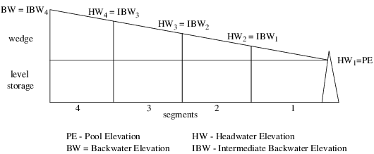
The Backwater Lambda LP Parameters (BLLPP) table is the only slot requiring user input, other than the physical data required to solve SlopePowerReservoirs with the Simulation controller. At least one realistic Headwater Elevation must be specified in the BLLPP table. Also at least one Inflow and/or Outflow for each segment is required, depending on the Reservoir’s configuration. The maximum and minimum Hydrologic Inflows during the run are automatically considered as potential Lambda Coefficients in addition to any user input Hydrologic Inflows in the BLLPP table. A lambda point is computed by RiverWare for every possible combination of Parameter values in the table columns. If a combination of values does not correspond to a feasible operational state, it is omitted from consideration. In certain cases, however, Inflow, Outflow, or Hydrologic Inflow values may not be required; the irrelevant columns in the BLLPP table are then omitted from the lambda point calculation. If any values are input into irrelevant columns, a warning message is issued at run time. The cases for which values are not required are:
Inflow is unnecessary if the a Profile Coeff Table parameter is zero for all segments. In this case, Inflow does not influence the backwater curve.
Outflow is unnecessary if the b Profile Coeff Table parameter is zero for all segments. In this case, Outflow does not influence the backwater curve.
Hydrologic Inflows are unnecessary if either the a or the wc Profile Coeff Table parameters are zero for all segments. In this case, Hydrologic Inflows do not influence the backwater curve. The minimum and maximum values are not treated as Lambda Coefficients.
The computed Lambda Points are stored in the Backwater Lambda Coefficients (BLC) table. The first columns of the table correspond to the Coefficients from the BLLPP table plus additional columns for time lagged Inflows and Outflows. The number of Inflow and Outflow columns is determined by the number of impulse response coefficients in the Profile Coeff Table. The remaining columns in the BLC table are the calculated Optimization parameters: Storage, Backwater Elevation, and Intermediate Backwater Elevations for each reservoir segment. Every row in the BLC table represents a valid lambda point. There is a row for each possible combination of Lambda Coefficients, including the lagged flows. The number of lambda point rows grows very quickly when multiple time lag columns compound the combinations. Since an excessive number of lambda points is unnecessary and affects performance, the number of lambda points is limited to 1,000.
The lambdaMethod uses the following slots in addition to those required for backwater calculation with the Simulation Controller:
Slots with Required Input Data
• Backwater Lambda LP Parameters (backwaterLambdaLPParms)
– TableSlot
– LENGTH, FLOW, FLOW, FLOW for each segment...
– valid operating points
– At least one Headwater Elevation is required. Inflow, Outflow, and Hydrologic Inflows may be required dependent on Reservoir configuration.
Slots with Output Data
• Backwater Lambda Coefficients (backwaterLambdaCoeffs)
– TableSlot
– LENGTH, FLOW for each irc..., FLOW for each irc..., FLOW for each segment..., LENGTH, LENGTH for each segment-1..., VOLUME
– a list of every combination of the valid operating points
Infeasible Solution Output File
RiverWare now automatically creates an output file when an infeasible optimization model is run. The file, called OPT_cplex_prob.*.iis, contains the “irreducibly inconsistent set” which represents the smallest infeasible problem from the failed run. This is typically a small set of inconsistent equations from which the erroneous constraint(s) can be deduced. The generation of this file is accompanied by a message window, indicating the exact name and path of the output file.
Optimization Output Files Directory
RiverWare-generated optimization files which begin with OPT_ are no longer saved in the RiverWare executable directory. All of these files, including those selected in the Optimization Controller Parameters dialog, are now saved in a sub-directory tree designed to facilitate management of this important debugging information.
The directory into which the files are saved is determined as follows:
• The top-most directory below which files are saved is either:
– the directory specified by the RiverWare_OPT_DIR environment variable,
– or the /tmp directory of the machine on which RiverWare is running.
Within this directory, a sub-directory is created as:
• the prefix “opt-” followed by the login name of the user.
(User johndoe would automatically generate a directory called opt-johndoe.)
Within this directory, an optional sub-directory may be created as:
• the File Directory: specified in the Optimization Controller Parameters dialog, if any.
For example: user johndoe running optimization with the RiverWare_OPT_DIR environment variable set to /RiverWare/Optimization, and the File Directory: set to run1, would generate OPT_ files as:
/RiverWare/Optimization/opt-johndoe/run1/OPT_*
If the File Directory: were then deselected, and the RiverWare_OPT_DIR environment variable were unset, OPT_ files would be generated as:
/tmp/opt-johndoe/OPT_*
In all cases, the directory to which optimization files are written is displayed as a green highlighted message in the Diagnostics Output Window.
Optimization Parameters Files
The PrsymOptParams file which contained optimization parameters for versions of PRSYM, has been divided into two files. The optimization parameters which are used exclusively by RiverWare are now contained in a file called goals.par. The optimization parameters which are required by the CPLEX solver are now contained in a file called cplex.par. The cplex.par file is passed directly to the solver as a command line argument, allowing a solution to be duplicated outside of the RiverWare executable. This is useful to access solver debugging capabilities which are unavailable during a RiverWare run.
The CPLEXPARFILE environment variable must be set as the path to the cplex.par file in order for this file to be located by the CPLEX solver. The path may be specified as an absolute path or a relative path from the directory set as the RiverWare_HOME environment variable.
Curvature Checks of Linearized Functions
Multiple term (MTLE & MTGE) Piecewise linearized functions are now checked for consistent curvature during Optimization runs. Violation of concavity or convexity is indicated by a warning message of the type:
SLOT(S): BlueRidge.Spill Bounds Linearization Table
“The value in row 48 column 1 (1796.703916) is outside the range of the approximation points and should be greater than the piecewise approximation (y = 9486.820540) for convex functions.”
The check to ensure that convexity or concavity is preserved is performed given the user approximation points, piecewise slopes, intercept, number of user approximation points, and the linearization context class of each table. The appropriate curvature is dependent upon the context, where MTLE and MTGE cases should yield convex and concave functions, respectively.
Two dimensional table values are checked by substituting the independent value into the piecewise function where the corresponding dependent value is computed. Since three-dimensional tables are linearized with respect to only one z point, their values are checked by examining independent values which are greater and less than the specified z point wherever an interpolation for the z approximation point is required. This provides a means with which to check for erroneous data which could potentially be used during actual interpolation. The appropriate independent values are then checked by substitution into the piecewise function where the corresponding dependent value is computed.
For both two-dimensional and three-dimensional tables, the dependent value is then compared to the table value to determine if the expected curvature is violated. In addition, piecewise slopes are checked relative to one another; convex and concave functions should yield slopes which are increasing and decreasing relative to one another, respectively.
RuleBased Simulation
Mass Balance Functions
There is now the ability for Rulebased Simulation to solve mass balances on Reservoir objects at any timestep. This was accomplished by adding three new mass balance methods on the Reservoir class that can be called from within a rule:
Reservoir:massBalanceSolveInflow (double out, double stor, double storPrev, Date_Time *dateTime, double &in)
Reservoir:massBalanceSolveOutflow (double in, double stor, double storPrev, Date_Time *dateTime, double &out)
Reservoir:massBalanceSolveStorage (double in, double out, double storPrev, Date_Time *dateTime, double &stor)
These functions differ from the standard massBalance functions in that they solve for the desired value in two steps. First, the given Inflow, Outflow, or Storage, as well as the Previous storage, and the time step (variables in, out, stor, storPrev, dateTime) provided by the Rulebased Simulation are converted to local variables of the MethodInfo class. Then, these functions execute the standard Reservoir:massBalanceSolve... (MethodInfo *LocalInfo) function which solves the mass balance. This standard method is the one used in the regular Simulation mode. The value computed by the massBalanceSolve... (MethodInfo *LocalInfo) function is then passed back to the rule as the desired &in, &out, or &stor.
Tcl Aggregation Functions
Several new Tcl-based functions have been added to the RuleBased Simulation language which access the new SubBasin functionality from within rules. They are:
C_GetAllNamedBasins
• This function returns a list of all user-defined SubBasins for the current model.
C_GetObjectsInBasin basinDesignator
• This function returns a list of all Objects in the SubBasin basinDesignator.
C_AggOverTime basinDesignator slotName aggFunc aggFilter scale units <startDate <endDate>>
• This function returns a list of values and their context(s). Each object in the designated basin is individually aggregated over time, yielding one item of the list. The type of the values, and the number of contexts returned, are determined by the Aggregation Function.
C_AggOverObj basinDesignator slotName aggFunc aggFilter scale units <startDate <endDate>>
• This function returns a list of values and their context(s). All of the objects in the designated basin are aggregated for each time, yielding one item of the list. The type of the values, and the number of contexts returned are determined by the Aggregation Function.
C_AggOverTimeObj basinDesignator slotName aggFunc1 aggFunc2 aggFilter scale units <startDate <endDate>>
• This function returns a single value and appropriate context. Each object in the designated basin is individually aggregated over time according to aggFunc1. The resulting list of objects are then aggregated according to aggFunc2. The value and number of contexts returned are determined by the Aggregation Functions (see table below).
C_AggOverObjTime basinDesignator slotName aggFunc1 aggFunc2 aggFilter scale units <startDate <endDate>>
• This function returns a single value and appropriate context. All of the objects in the designated basin are aggregated according to aggFunc1 for each time. The resulting list of times are then aggregated according to aggFunc2. The value and number of contexts returned are determined by the Aggregation Functions.
Where the arguments to the above functions are specified as:
– basinDesignator:
– {basinName}
– {basinName {classType}}
– {direction refObject}
– {direction refObject {classTypes}}
– {direction refObject {classTypes} {terminators}}
– {direction refObject {classTypes} {terminators} {in/excludedBasins}}
– basinName:
– Any user-defined or RiverWare-defined basin.
– classTypes:
– AggDiversionSite
– AggReach
– Canal
– Confluence
– GroundWaterStorage
– LevelPowerReservoir
– PowerReservoir
– PumpedStorage
– Reach
– Reservoir
– SlopePowerReservoir
– StandAloneWU
– StorageReservoir
– Thermal
– WaterUser
– direction:
– UPSTREAM
– DOWNSTREAM
– refObject:
– An object name.
– terminators:
– Object name(s).
– in/excludedBasins:
– Any user-defined or RiverWare-defined basin(s)
– aggFunc:
– SUM
– AVG
– MIN
– MAX
– aggFilter (filters out all which are not flagged):
– IN_OUT
– INPUT
– OUTPUT
– <startDate>:
– An optional starting dateTime. If not specified, defaults to the current dateTime.
– <endDate>:
– An optional ending dateTime, only valid if <startDate> is also specified. This also defaults to the current dateTime.
AggFunc | C_AggOverObj | C_AggOverTime |
|---|---|---|
MIN or MAX | Returns {objectName dateTime value} for each dateTime in the range | Returns {objectName dateTime value} for each object in the SubBasin |
SUM or AVG | Returns {dateTime value} for each dateTime in the range | Returns {objectName value} for each object in the SubBasin |
AggFuncs | C_AggOverObjTime | C_AggOverTimeObj |
|---|---|---|
MIN or MAX, then MIN or MAX | Returns a single {objectName dateTime value} | Returns a single {objectName dateTime value} |
MIN or MAX, then SUM or AVG | Returns a single {value} | Returns a single {value} |
SUM or AVG, then MIN or MAX | Returns a single {dateTime value} | Returns a single {objectName value} |
SUM or AVG, then SUM or AVG | Returns a single {value} | Returns a single {value} |
Note: If an aggregate cannot be computed due to an invalid value in one of its items, the returned value will be “NaN” and the returned date, if applicable, will be “NO_DATE.” All aggregations are done in standard units. Values in units of acre-feet/month are NOT scaled to the length of each dateTime in the range. As such, their results will be invalid for any dateTimes which are not 31 days long.
Tcl Unit Conversion Functions
Two new functions have been added to facilitate unit conversions. They are:
C_GetStepSeconds <dateTime>
• This function returns the number of seconds in the timestep referenced by <dateTime>. If no <dateTime> is specified, the current dateTime is used. The number of seconds in the timestep may be used to convert between units of FLOW and VOLUME within rules.
C_ConvertValue fromValue fromScale fromUnits toScale toUnits <dateTime>
• This function converts a given fromValue with scale and units of fromScale and fromUnits, to a value in the scale and units of toScale and toUnits. All conversions must be within a single unit type; e.g., FLOW. The optional <dateTime> specification indicates the timestep who’s length will be used for conversions from/to units of acre-feet/month. If no <dateTime> is specified, the current dateTime is used.
Total Diversion to Meet Requests
A new function has been added which computes the Diversion required to satisfy the Diversion Requests of all WaterUsers of an AggDiversionSite at any timestep of the simulation. This function may be called from within a rule for AggDiversionSites using the Sequential Linking Structure only. In order to perform the calculation, the algorithm executes the selected returnFlowCalculation and returnFlowSplitCalculation Methods on each WaterUser. These account for all possibilities of Return Flow linking and quantities when computing the variable totalReq, which represents the Diversion requirement for satisfaction of all WaterUser requests. The function is defined as:
int nonShortDiversionReq(double &totalReq, Date_Time *when)
where totalReq is the calculated total Diversion and when is a pointer to the timestep at which the calculation is to be performed. The function returns 0 upon success and 1 upon failure.
GUI
Toolbar
A toolbar has been added to the main RiverWare Workspace window. It contains buttons for accessing commonly used commands and dialogs. The buttons are:
• Load Model File This button is equivalent to Model Load... or <Ctrl> L.
• Save Model File This button is equivalent to Model Save... or <Ctrl> S. (See Model Loading and Saving for details on the new implementation of the Save command.)
• Run Control Panel This button is equivalent to Control Run Control Panel... or <Ctrl> R.
• MRM Control Panel This button is equivalent to Control MRM Control Panel... or <Ctrl> M.
• Object Palette This button is equivalent to Workspace Object Palette... or <Ctrl> P.
• Link Editor This button is equivalent to Workspace Link Editor... or <Shift> E.
• Locator View This button is equivalent to Workspace Locator View... or <Shift> V.
• Edit SCT This button is equivalent to Utilities Edit SCT....
• Unit Converter This button is equivalent to Utilities Unit Converter....
• Snapshot Management This button is equivalent to Utilities Snapshot Management....
• Plotting Management This button is equivalent to Utilities Plotting Management....
• Dispatch Information This button is equivalent to Utilities Dispatch Information....
Keyboard Shortcuts
Many of the keyboard shortcuts for commonly used commands have been modified to be consistent between different RiverWare dialogs, to conform to accepted software standards, and to eliminate conflicts arising from duplicate shortcuts. In dialog menus, keyboard shortcuts appear to the right of the commands they execute. The shortcuts are:
Shortcut | Corresponding Menu Function |
|---|---|
Ctrl + L | Model Load... |
Ctrl + S | Model Save |
Ctrl + Shift + S | Model Save As... |
Ctrl + R | Control Run Control Panel... |
Ctrl + M | Control MRM Control Panel... |
Ctrl + Shift + E | Control Reevaluate Expression Slots |
Ctrl + O | Workspace Open Object(s) |
Ctrl + - | Workspace Delete Object(s) |
Shift + P | Workspace Object Palette... |
Ctrl + Shift + L | Workspace Link Editor... |
Ctrl + Shift + B | Workspace Edit SubBasins... |
Ctrl + B | Workspace List SubBasin Membership |
Shift + L | Workspace Locator View... |
Ctrl + Shift + R | Policy Rules Interface... |
Ctrl + Shift + C | Policy Constraint Editor... |
Shortcut | Corresponding Menu Function |
|---|---|
Ctrl + H | Special Home |
Ctrl + M | Special Mark |
Shortcut | Corresponding Menu Function |
|---|---|
Ctrl + W | File Close Window |
Shortcut | Corresponding Menu Function |
|---|---|
Ctrl + S | View Run Status Dialog |
Shortcut | Corresponding Menu Function |
|---|---|
Ctrl + Shift + S | View Slot Lists |
Shortcut | Corresponding Menu Function |
|---|---|
Ctrl + L | File Load Slot List |
Ctrl + S | File Save Slot List |
Ctrl + Shift + S | File Save As |
Shortcut | Corresponding Menu Function |
|---|---|
Ctrl + L | File Load Run List |
Alt + Plus | Edit Insert Run Before |
Ctrl + Plus | Edit Append Run |
Ctrl + Minus | Edit Delete Run |
Shortcut | Corresponding Menu Function |
|---|---|
Alt + A | Edit Add Time Horizon |
Alt + Plus | Edit Insert Time Horizon |
Ctrl + Minus | Edit Delete Time Horizon |
Alt + D | Edit Clear |
Shortcut | Corresponding Menu Function |
|---|---|
Ctrl + Shift + S | View Slots |
Ctrl + Shift + M | View Methods |
Ctrl + O | Slots Open Slot |
Shortcut | Corresponding Menu Function |
|---|---|
Ctrl + I | File Import (Resize) |
Ctrl + Shift + I | File Import (Fixed Size) |
Ctrl + E | File Export |
Ctrl + X | Edit Cut Row or Edit Cut Cell |
Ctrl + C | Edit Copy Row or Edit Copy Cell |
Ctrl + Minus | Edit Delete Row or Edit Delete Cell |
Ctrl + Shift + V | Edit Insert Cut/Copied Row |
Ctrl + V | Edit Paste Cut/Copied Cell |
Alt + Plus | Edit Insert New Row Before or Edit Insert New Cell Before |
Ctrl + Plus | Edit Append New Row or Edit Append New Cell |
Ctrl + D | Edit Fill Values Below |
Ctrl + Shift + D | Edit Set Dimensions |
Ctrl + A | Edit Select All |
Ctrl + U | Edit Unselect All |
Alt + Shift + C | View Configuration |
Ctrl + Shift + E | View Expression Editor |
Alt + I | TimeStep I/O Input |
Alt + O | TimeStep I/O Output |
Ctrl + T | TimeStep I/O Target |
Ctrl + B | TimeStep I/O Best Efficiency |
Ctrl + M | TimeStep I/O Max Capacity |
Ctrl + Tilde | TimeStep I/O Drift |
Shortcut | Corresponding Menu Function |
|---|---|
Alt + Plus | SubBasin Insert New Before |
Ctrl + Plus | SubBasin Append New |
Ctrl + U | SubBasin Update From Workspace |
Ctrl + L | Object List SubBasin Membership |
Shortcut | Corresponding Menu Function |
|---|---|
Ctrl + L | Rule Set Clean Load |
Ctrl + B | Rule Set Clear |
Ctrl + C | Rule Set Close |
Ctrl + S | Edit/View Rule Set |
Ctrl + R | Edit/View Rules |
Ctrl + A | Edit/View Agenda |
Ctrl + D | Edit/View Dependencies |
Ctrl + P | Interact Breakpoints |
Ctrl + X | Interact Execute Rule |
Shortcut | Corresponding Menu Function |
|---|---|
Ctrl + O | Edit Display/Hide Sub-rows |
Ctrl + E | Edit Edit File |
Shortcut | Corresponding Menu Function |
|---|---|
Ctrl + R | Edit Reset Agenda |
Ctrl + E | Edit Edit File On Agenda |
Ctrl + F | Edit Edit File Off Agenda |
Shortcut | Corresponding Menu Function |
|---|---|
Ctrl + E | Breakpoints Edit/Add |
Del | Breakpoints Delete |
Ctrl +B | Breakpoints Delete All |
Shortcut | Corresponding Menu Function |
|---|---|
Ctrl + L | File Load Constraint Set |
Ctrl + Plus | File Append Constraint Set |
Ctrl + S | File Save Constraint Set |
Ctrl + N | Edit Add Constraint |
Alt + Plus | Edit Insert Goal |
Ctrl + A | Edit Add Goal |
Ctrl + G | Edit Add Group |
Ctrl + Minus | Edit Delete |
Ctrl + H | Edit Change Priority Level |
Alt + P | Edit Pack Constraint Set |
Ctrl + Shift + E | View Open Expression Editor |
Shortcut | Corresponding Menu Function |
|---|---|
Ctrl + I | Values Set Input |
Ctrl + V | Values Set Input Values |
Ctrl + T | Values Set Detail Values |
Ctrl + O | Values Set Output |
Ctrl + C | Values Clear Output |
Ctrl + Z | Values Target Operation |
Ctrl + B | Values Best Efficiency |
Ctrl + M | Values Max Capacity |
Ctrl + Tilde | Values Drift |
Ctrl + S | Values Summary Type... |
Ctrl + F | View Refresh |
Ctrl + D | Run Run Control Dialog... |
Ctrl + R | Run Start Run... |
Shortcut | Corresponding Menu Function |
|---|---|
Ctrl + X | Data Cut |
Ctrl + C | Data Copy |
Ctrl + V | Data Paste |
Alt +D | Data Clear |
Ctrl + A | Data Select All |
Alt + A | Data Add Data... |
Shortcut | Corresponding Menu Function |
|---|---|
Ctrl + N | Plot Page New... |
Ctrl + O | Plot Page Open... |
Ctrl + Minus | Plot Page Delete |
Ctrl + F | Refresh Refresh Plot Page |
Ctrl + A | Refresh Refresh All Plot Page |
Shortcut | Corresponding Menu Function |
|---|---|
Ctrl + N | Plot Page New... |
Ctrl + O | Plot Page Open... |
Ctrl + Shift + S | Plot Page Save As... |
Ctrl + F | Plot Page Refresh |
Ctrl + X | Data Cut |
Ctrl + C | Data Copy |
Ctrl + V | Data Paste |
Alt + D | Data Clear |
Ctrl + A | Data Graph All |
Ctrl + Shift + S | Data Select Slots... |
Shortcut | Corresponding Menu Function |
|---|---|
Ctrl + E | Object Enable Dispatching |
Ctrl + D | Object Disable Dispatching |
Shortcut | Corresponding Menu Function |
|---|---|
Ctrl + L | File Load Settings... |
Ctrl + S | File Save Settings... |
Shortcut | Corresponding Menu Function |
|---|---|
Ctrl + L | File Load Settings... |
Ctrl + S | File Save Settings... |
Shortcut | Corresponding Menu Function |
|---|---|
Alt + O | Select All Objects |
Alt + S | Select All Slots |
Alt + R | Select All Rules |
Alt + N | Select All Constraints |
Alt + G | Select All Goals |
Alt + T | Select All Times |
Alt + D | Select All Diagnostics Groups |
Alt + A | Select All All |
Shift + O | Revert Objects |
Shift + S | Revert Slots |
Shift + R | Revert Rules |
Shift + N | Revert Constraints |
Shift + G | Revert Goals |
Shift + T | Revert Times |
Shift + D | Revert Diagnostics Groups |
Shift + A | Revert All |
Ctrl + O | Clear Objects |
Ctrl + S | Clear Slots |
Ctrl + R | Clear Rules |
Ctrl + N | Clear Constraints |
Ctrl + D | Clear Diagnostics Groups |
Ctrl + A | Clear All |
Shortcut | Corresponding Menu Function |
|---|---|
Ctrl + S | File Save To File... |
Ctrl + L | File Legend |
Ctrl + R | File Clear |
Ctrl + I | Find String... |
Pinnable Menus
The main RiverWare Workspace menus are now pinnable. Clicking on the dashed line at the top of an open menu converts the menu into a free window. This allows repeated commands to be executed without first having to re-open the menu. To close a pinned menu, kill the Xwindows frame in which it resides by clicking twice on the upper left corner of the window.
Default Window Placement
The placement and size of the main Workspace window is now preserved from one RiverWare session to the next. The location in the Xwindows monitor and the size of the window are saved in the.vgalaxy.1.vr file in the user’s home directory. The placement and location are applied when the RiverWare executable is initially launched and are then automatically saved from the current configuration when the session is ended.
Locator View
A new function has been added to facilitate movement around the workspace of large models. Selecting the Locator View... command from the Workspace menu creates a miniature representation of the entire workspace in a new window. A highlighted frame indicates the portion of the workspace over which the main RiverWare window is currently located. Dragging this frame to a different part of the workspace shifts the main RiverWare window’s field of view to match the locator. A specific object may be also be brought into view by selecting it from the Locate menu heading on the locator window.
View Methods/Slots
The View Methods and View Slots buttons on the Open Object dialog have been converted to an option menu. This menu is labeled as View:. It indicates the currently selected dialog view from two options, Slots and Methods. Slots view is the default.
SubBasins
A SubBasin is a collection of workspace simulation objects which are grouped under a single name. For example, it may be convenient to specify a SubBasin named “Main River” whose members are all of the Reach and Reservoir objects along the main stem of a riverbasin. The name of the SubBasin may then be used to efficiently represent all of its member objects in calculations. Currently, the use of SubBasin names is only supported for Expression Slots and Optimization Constraints. This functionality will be expanded to the Rulebased Simulation Structured Editor in upcoming releases.
SubBasins and their memberships are set through the SubBasin Manager. This dialog is invoked by selecting Edit SubBasins... from the Workspace menu heading. The default SubBasin is the “Entire Network.” This SubBasin may not be deleted, modified, or renamed. It contains all of the objects on the workspace with the exception of Data Objects. Data Objects may never be included in any SubBasin membership.
Selecting the tree-view arrow to the left of a SubBasin name will display the list of its members. If any Aggregate Objects are members of the SubBasin, selecting the tree-view arrow to the left of their name(s) will display a list of their member Elements. Each of these Aggregate Elements is included in the SubBasin. Elements may not be individually included or excluded from a SubBasin definition. The name of a SubBasin may be changed by selecting its existing name and typing a new name into the resulting edit window. The commands available from the Edit SubBasins dialog are:
File Close to close the SubBasin Manager dialog. This is the same as clicking the Close button at the bottom of the dialog.
SubBasin Insert New Before to define a new SubBasin with the selected objects on the workspace and to insert the name before the currently highlighted SubBasin name.
SubBasin Insert New After to define a new SubBasin with the selected objects on the workspace and to insert the name after the currently highlighted SubBasin name.
SubBasin Append New to define a new SubBasin with the selected objects on the workspace and to insert the name at the end of the SubBasin list.
SubBasin Update From Workspace to redefine the currently highlighted SubBasin. The membership will be cleared and replaced by the selected objects on the workspace.
SubBasin Select on Workspace to highlight the members of the currently selected SubBasin on the workspace.
Object List SubBasin Membership to bring up a new window displaying the SubBasin(s) to which the selected object belongs.
The Remove button will delete the currently selected SubBasin or member.
The Close button closes the SubBasin Manager dialog.
An object’s membership may also be directly displayed without invoking the Edit SubBasins dialog. To do this, first highlight a single object on the workspace. Next, select Workspace List SubBasin Membership from the main RiverWare menu bar. A new window appears listing all SubBasins to which the selected object belongs.
SCT
Set Row Type Dialog
The dialog for determining which slot is displayed in an SCT row has been updated. Selecting Rows Set Slot... now brings up the SCT Row Type slot selector only if there are objects on the workspace. The Object types: option menu has been improved to list only the object types of which at least one member exists on the workspace. These object types are listed in alphabetical order. To facilitate building an SCT, the SCT Row Type dialog is invoked with a default selection corresponding to the object and slot of the last row to have been configured. This allows many rows to be assigned to slots on the same object without having to reselect the object type and object for each occurrence.
Toggle Row Detail in non-Edit Mode
The view of row detail values may now be toggled when Editing: is turned OFF. This provides access to detail timesteps for changing their values. The summary type of a row’s detail values may also be changed by selecting Values Summary Type.... These additional functions provide flexibility in non-Edit mode, while safeguarding the configuration of the original SCT.
Setting of Closed Detail Values
Setting detail values in a closed row through the Values Set Detail Values command is no longer supported. This functionality was dangerous, as it allowed values and flags to be overwritten without any visual confirmation of the effects. Detail rows must now be open for this command to be enabled. The old behavior will continue to exist in SCTs until the first time their rows are toggled and the SCT is saved.
DMI
DMI Generated Error Messages
Although DMIs may now exit with a -1 return status, DMI generated error messages will not be properly interpreted by RiverWare. For proper handling of errors and messages, the accepted exit codes are:
• 0 Success
• 1 - 127 Error
New Keyword=Value Pair: Flags
Valid keyword=value pairs have been expanded to include flags. This keyword can enable the importing or exporting of the SeriesSlot flags at every timestep, in addition to the slot values. The possible values for this keyword are true and false.
A keyword=value of the type:
flags=true
will cause SeriesSlot flags (INPUT, OUTPUT, TARGET, TARGET_BEGIN, BEST_EFFICIENCY, MAX_CAPACITY, and DRIFT) to be imported or exported with the data. This is an optional keyword=value pair which defaults to false if not specified.
Values in User-defined Keyword=Value Pairs
Values may no longer include spaces ( ), colons (:), or exclamation points (!). Due to changes in the parsing of DMI control files, these characters are now used as delimiters. Their use within a value field will cause a syntax error and prevent proper execution of the DMI. As there are no known DMIs currently using this punctuation, the change should not affect any existing models.
Control File Object and Slot Wildcards
Control File Object and Slot Wildcards have been expanded to include subBasins and dispatch slots, respectively. An object.slot specification of the type:
<basinname>.<slot>
will match any <slot(s)> within the subBasin <basinname>. Similarly, an object.slot specification of the type:
<object>.dispatch
will match any dispatching slot in the given <object(s)>. These new object.slot wildcards may be used in conjunction with the flags=true optional keyword=value to import or export all of the values and flags for the dispatching slots of a subBasin. This type of DMI allows the information required to uniquely reproduce a scenario to be moved between subBasins of different models. For more information on using DMIs towards this end, contact CADSWES staff.
RCL and Batch Mode
Rulesets for Rulesbased Simulation
Rulesets for Rulebased Simulation may now be loaded using the RiverWare Command Language. The syntax for this new command is:
LoadRules ruleset
where ruleset is a valid file pathname to a ruleset.
Expression Slots
Overview of Functionality
Functionality has grown extensively over the past several releases. In order to put new features into perspective, an overview of the existing state of the expression slot is presented here.
To create a new expression slot, open a Data Object and select Slots Add Expression Slot. The new slot is appended to the slot list with the name ExpressionX (where X is the smallest integer needed to make this name unique, beginning with 00000), and marked with the expression icon above. To open an expression slot, double-click on its name.
Expression Slots may be renamed through the Name: field in the Open Slot dialog. Expression Slots are initially created with the Run Control’s Initial: time only. When the expression is evaluated, the time range of the slot is expanded to mirror the time horizon in the Run Control dialog.
The units and Display Units label, scale, and precision of values displayed as the result of an Expression Slot may be changed through the Configuration menu. Expression Slots may display all RiverWare defined unit types, but default to a unit type of NONE. When the NONE unit type is selected, a Display Units field is available to enter a display label. This label is saved in the model file, but is not exported through DMIs in the same manner as RiverWare defined units. Any Expression Slots with Unit Type of NONE is written to DMIs with User Units of NONE. The label is only cosmetic, and in no way affects the calculation of the expression or scaling of the display value. When a unit type other than NONE is selected, an option menu appears for the user to select a RiverWare defined unit. These units ensure a consistency of labeling for exported data.
Expressions are only calculated based on the display values of the slots they reference. No attempt is made to reconcile varied units or carry them through an expression. The user is responsible for verifying that display values in referenced slots are consistent with the nature of the expression. Unit conversions may be performed after an Expression Slot has computed, by changing the Expression Slot’s units in the Configuration menu. Any such conversion will only be performed when changing from one RiverWare defined unit to another. The converted value is retained only as long as the Expression is not recalculated. When the expression is recalculated, the computed value will be assumed to be in the currently selected units.
The expression itself is displayed in the scrollable Expression: window. To create a new expression, select the Editor button or select View Expression Editor. The Expression Editor is a syntax-directed editor designed to assist in the construction of complex syntactically correct expressions within the RiverWare environment. The editor works by maintaining a partially constructed expression and allowing the user to manipulate unfinished portions using a collection of selection lists and text entry boxes. To use this dialog effectively, it is important to formulate the expression in its entirety (perhaps on paper) before beginning. The Expression Editor does not allow editing of previously determined portions of the expression. Errors in specifying an expression must be corrected by clearing the existing expression and beginning anew.
Initially, the editor contains a single ? indicating a portion of an expression which has not yet been completed. Clicking, without releasing, on the ? brings up a term selection list. Scrolling down to a term and releasing the mouse, inserts the selected term in place of the ?. Terms may contain additional ?s, to expand the complexity of the expression. One of two selection lists is available from any ?. These fall into two categories: General Terms and Range Terms. General Terms include algebraic manipulations, variables (slots and user-defined variables), and actual values. Range Terms indicate the range over which an expression is computed. This may be a collection of slots, a SubBasin, or a set of timesteps.
Term | Significance |
|---|---|
? + ? | Addition |
? - ? | Subtraction |
? * ? | Multiplication |
? / ? | Division |
(?) ^ (?) | Exponentiation |
( ? ) | Parenthetical grouping |
NUMBER | Numerical input; Selecting NUMBER opens a text entry field. |
Note: Operator precedence is as follows (greatest to least): (), ^, * and /, and + and -. Parenthetical notation is automatically added to an expression when it is committed. This alleviates any later confusion regarding under-specified operator precedence.
Term | Significance |
|---|---|
“SLOT” [ @t ] | Slot value at time of expression. |
“SLOT” [ @t - NUMBER] | Slot value at offset from time of expression; the offset should be an integer number. |
“SLOT” [ ? ] | Slot value at time ? Clicking on ? opens an entry field for a variable. |
Note: Selecting “SLOT” opens a slot selector dialog for selection of Object-Slot combinations in one of three ways:
• Selecting a black-lettered object in the Objects: column generates a list of all of its slots in the Slots: column. Selecting one of these slots and pressing the OK button concludes the selection. The chosen slot, referenced according to standard “object.slot” notation, is visible in the Selected Slot: field.
• Selecting a blue-lettered object type in the Objects: column generates a list of slots in the Slots: column which exist for every object of that type. Selecting one of these slots and pressing the OK button concludes the selection. The chosen slot(s) will appear as “@Var.slot” in the Selected Slot: field, where “Var” is a three letter variable representing the object type. This style of entry is useful for expressions which require iterating over every object of a given type.
• An “object.slot” may be typed directly into, or a partial selection may be edited directly in, the Selected Slot: field. This style of entry is useful to specify custom variables for iterations such as “@Var.slot.” In this case, Var must be defined elsewhere in the expression.
Term | Significance |
|---|---|
S [ ? , ? ] | Sum second ? over range of first ?. |
X [ ? , ? ] | Average second ? over range of first ?. |
S [ ? IN ? , ? ] | Sum last ? over subset of first ? in range of second ?. |
X [ ? IN ? , ? ] | Average last ? over subset of first ? in range of second ?. |
Note: The final ? of summation and average terms may be replaced by any Algebraic Terms, Slot References, or Iteration Operators. The latter results in nested loops. The ? IN ? range terms are useful for specifying a different variable than that automatically provided by a simple ? Range Term. If ? IN ? is selected as a term, the first ? opens a text entry field for entering a user variables, while the second ? produces a list of terms “over which” to range.
Term | Significance |
|---|---|
t IN Time | t ranges over all simulation timesteps |
t IN Time ? | t ranges over the Time Subset ? of all simulation timesteps. |
i IN Integer FROM ? TO ? | i ranges over all integers from ? to ?. |
i IN Integer FROM ? TO ? INC ? | i ranges over all integers from ? to ? in increments of ?. |
Var IN “SubBasin” | Var ranges over all the objects within SubBasin. |
Note: If the difference between the FROM and TO values is not an integer multiple of the INCrement, the TO value will not be considered within the range. Multiple Var IN “SubBasin” Range Terms are automatically appended to the list to represent every SubBasin on the workspace. Both user-defined and internally-defined SubBasins appear in the list. The Var variable name is composed of the first three letters of the SubBasin name.
Term | Significance |
|---|---|
BY “SLOT” | Includes only timesteps where “SLOT” has a valid value. |
FROM ? TO ? | Includes all integers from ? to ?. |
FROM ? TO ? INC ? | Includes all integers from ? to ? in increments of ?. |
FROM ? | Includes all integers from ?. |
TO ? | Includes all integers to ?. |
? ? | Creates multiple Time Subsets. |
Note: Multiple Time Subsets may be used to increment over integers which are themselves increments.
Term | Significance |
|---|---|
@? | Value at variable time ?; Selecting ? opens an entry field for the variable name. |
Note: All variables used in expressions must be defined within that expression.
SubBasins
Expression slots have been expanded to utilize the new SubBasin functionality previously described. It is now possible to iterate over user-defined SubBasins as well as object types. SubBasins will appear in the expression editor’s menu list when summing or averaging values. Note that any change in the membership of a SubBasin will be reflected in the calculations of any Expression Slots which reference it.
Linking
Expression slots may now be linked to other slots on the workspace. This is useful for propagating a set of calculated values into a dispatching Series Slot prior to simulation. Propagation across a link occurs every time an Expression slot is reevaluated, which may be done outside of a run by selecting Control Reevaluate Expression Slots from the main workspace menu bar, or by using the <Control>-e keyboard shortcut. Reevaluation of Expression slots may not be forced during a simulation run, but will still be done automatically at the conclusion of the run. Linking an Expression slot to a Simulation slot which receives a computed value during a run will cause an error and abort the run when the value propagates to the expression slot.
Dispatch Information
A new Dispatch Information utility has been created to provide post-run diagnostics regarding object dispatching and known values of dispatching slots for every timestep of the simulation. The Dispatch Information dialog is invoked by selecting Dispatch Information... from the Utilities menu heading in the main RiverWare workspace window or by clicking on the Dispatch Information shortcut button on the toolbar.
The Dispatch Information tool provides dispatch information at two levels of detail. At the workspace level, the dispatch state of each object for each timestep of the model run is visible. At a more detailed level, the tool allows an object’s dispatch table entries and known slot values at the end of each timestep to be viewed.
Workspace-level View
The Dispatch Information dialog displays the workspace-level view of dispatch conditions. This dialog consists of a two-dimensional matrix with workspace objects on one axis and model run timesteps on the other axis. Each cell in the matrix shows the dispatch state of an object at the indicated timestep. Dispatch entries are made automatically during run initialization, so no dispatch information is available until a run is completed. Because they never dispatch, Data Objects and Snapshot Objects are not included in the list of Objects. An Object has one of four possible dispatch states:
Not Dispatched. The known and unknown slots for the timestep did not meet the requirements of any method on the dispatch table for the Object.
Dispatched. Conditions of a single method on the dispatch table were met; the method dispatched, and the Object solved.
Dispatched But Not Solved. Conditions of a single method on the dispatch table were met; the method dispatched, but the Object did not solve completely.
No Dispatch Entries. The Object has no entries on its dispatch table; the Object is a Thermal Object, or the model has not been run.
Selecting an Object/timestep cell displays its dispatch state in text form at the bottom of the Dispatch Information dialog. If the Object dispatched at that timestep, then the name of the method under which it dispatched is also displayed.
The Dispatch Information dialog may be reformatted from its original configuration. If the lists holding the names of Objects and timestep are too narrow to read, they may be expanded by clicking on the double-arrow buttons. This will alternately increase and decrease the size of the headers between an abbreviated length and one which accommodates the longest Object/timestep name. The view in the Dispatch Information dialog can also be transposed so that timesteps appear along the side of the dialog and Object names appear along the top. To transpose the view, select View Time On Side or View Time On Top from the menu bar.
Finally, the order in which Objects appear in the dialog may be rearranged from its original alphabetical order. This is useful to match the river topology or any order with which you are more familiar. To rearrange an Object, select its name with the middle mouse button and drag the resulting frame to a new location. Releasing the middle mouse button will place the Object just beyond the Object over which the frame is located; above when moving an Object up, below when moving an Object down.
Please note: new formats are only saved with the model file, so be sure to re-save the model after changing the Dispatch Information.
The Dispatch Information dialog may be used to disable or enable dispatching for individual Objects. Disabling dispatching prevents the object from dispatching at any timestep, regardless of what slots are known. This functionality is useful to debug models. To disable dispatching for an Object, select its name and select Object Disable Dispatching from the Dispatch Information dialog menu bar. The Object name is shaded with red diagonal lines to indicate that it will no longer dispatch. The Object’s Beginning of Run behavior, however, may never be disabled. To re-enable dispatching, select the name of the Object for which dispatching has been disabled and select the Object Enable Dispatching. The red diagonal lines disappear from the Object name, and it is allowed to dispatch when the model is run.
Dispatch Detail Dialogs
The Dispatch Detail dialogs allow the entries in the dispatch table and the known slots at the end of each timestep to be viewed for each object. To open a Dispatch Detail dialog, double-click on a cell in the Dispatch Information dialog which represents the desired object and timestep. One of the following occurs, depending on the dispatch state of the selection.
If the Object has no dispatch conditions, or the model has not yet been run, a warning message is displayed.
If the Object did not dispatch during the selected timestep, the Dispatch Detail dialog appears showing a list of slots. Each of the displayed slots is a required known and/or a required unknown for an entrie(s) in the Object’s dispatch table. The checkmarks indicate which slots were known at the end of the selected timestep.
• To view the entries in the dispatch table for this object, select Methods from the view option menu. The methods view lists all of the methods in the Object’s dispatch table, each marked with a symbol indicating whether the method dispatched. Since the object did not dispatch, none of the methods have a green D symbol. Selecting the, and sots in the list with a box to their left are required knowns for the method to dispatch. Slots with no box are required unknowns. Checkmarks indicate which slots were known at the end of the timestep.
If the object did dispatch during the selected timestep, the Dispatch Detail dialog appears showing a list of methods from that Object’s dispatch table. The method which dispatched at the selected timestep is marked with the dispatched symbol and is opened to show its dispatch conditions. Notice that all of the slots are checked as known, even those required to be unknown. This occurs because the object solved correctly for all slots, making them known by the end of the timestep. We know that the dispatch conditions requiring unknowns were met at the time of dispatching because the method could not have dispatched otherwise. This may seem slightly confusing, but remember that the known/unknown status of particular slots is truly of interest only if the object failed to dispatch at the selected timestep. If the object did indeed dispatch, all of the conditions must have been met.
In models with hourly, daily, or monthly timesteps, the Dispatch Detail dialog contains a date spinner which moves the detail view forward and backward over the range of the model run. Clicking on the up arrow of the date field spinner moves the dialog view one timestep forward in the run. Clicking on the down arrow moves the view one timestep backwards in time. This is useful to determine how the set of known slots changes from timestep to timestep.
Diagnostics
Scrollable Windows in the Diagnostics Output Window
The Diagnostics Output Window now contains windows for Contexts and Messages that are independently scrollable. The scroll bars along the bottom of each window may be used to view information which extends beyond their right borders. The scroll bar along the right side of the dialog scrolls both windows simultaneously. The width of each window may be modified by clicking in the space between the two headings and dragging the outline of the heading bars to the new desired location. Message lines are now separated by a horizontal rule to increase their legibility.
Diagnostics Output Efficiency
The Diagnostics Output Window has been reformatted to be more efficient. Display allocation in the window is now done in increments of 50 lines. This significantly decreases model run time when many diagnostics are enabled. This does not, however, completely alleviate the potential for “freezing” RiverWare when too many diagnostics are enabled. Users should still exercise prudence in selecting only the appropriate categories and filters for diagnostics.
Enabling Diagnostics
The name of the toggle for enabling diagnostics information has been changed from Include General Information to Enable Informational Diagnostics. As before, this toggle has no effect on Errors and Warnings produced during a run. Errors and Warnings are not user-configurable. They are always displayed in the Diagnostics Output Window, regardless of whether Informational Diagnostics are enabled.
Plotting and Snapshots
New functionality exists for saving and combining plots of output values from several different slots and runs. The Snapshot Management dialog is used to create and review snapshots of selected slot values over multiple runs.The Plotter Management dialog is used to create composite plots for display or printing.
The Snapshot Management Dialog
The Snapshot Management dialog is invoked by selecting Utilities Snapshot Management.... It allows snapshots of selected slot values to be taken after different runs. This tool is useful for saving the values to compare the effects of various operating strategies or reproduce a particular run.
Slots to be included in a snapshot are selected by clicking on the Add Data... button, which invokes a Slot Selector dialog. Newly selected slots are added to any existing slots in the Data Available: window. These selections may be cut, copied, pasted, and cleared through the Data menu. Slot selections may also be copied between the Snapshot Management and the Plotter Management dialogs. This greatly facilitates configuration of plots and preparation of snapshots for preconfigured plots.
Snapshots of the selected slots’ current values are taken by clicking on the Take Snapshot button. Each time a snapshot is taken, the Snapshot Manager creates a new Snapshot Data Object to contain its data. The new object is added to the bottom right of the workspace, and its name appears in the Snapshots Taken: window. Snapshot Objects are initialized with the name Snapshotn, where n is the smallest number, beginning with 0000, which makes the object name unique. The selected slots are copied into the Snapshot Object, retaining their unit and display configurations. These slots are initialized with the name of the object and the name of the slot from which they were copied, separated by an underscore. For example, a snapshot of the Inflow slot on the Big River Reach appears as “Big River_Inflow.” While snapshot slot names may not be changed, Snapshot Object names may be changed by entering a new name in their Name: field.
Selecting a selected slot name in the Data Available: window highlights any snapshot objects in the Snapshots Taken: window, which contain a snapshot of that slot. Double-clicking on a Snapshot Object name in the Snapshots Taken: window automatically brings up that Snapshot Object. Double-clicking on a selected slot name in the Data Available: window brings up that object and the slot’s current model values.
The Plotter Management Dialog
The Plotter Management dialog is invoked by selecting Utilities Plotting Management....
The Plotter Manager maintains a list of all existing Plot Pages, which may be created, opened, deleted and refreshed from this dialog. To create a new Plot Page, select Plot Page New..., or select the New... button. To open an existing Plot Page, highlight it and select Plot Page Open... or select the Open... button.
The Plotter dialog is used to select the number and orientation of graphs to be displayed on one page, as well as what slot data will appear in each individual graph. Plot Pages are initialized with the name Plottern, where n is the smallest number, beginning with 00000, which makes the Plot Page name unique.The plotter name is changed by typing into the Plot Page: field. The number and layout of graphs is selected through the Graph Layout: selector bar. Up to nine graphs may be generated on a single page, with graph layout referenced according to row-column notation. For example, a 2 x 1 layout consists of two rows with one graph per row. The layout is represented graphically in the Select Graph: region.
Individual graphs are selected by clicking on their icon in the Select Graph: region. Graphs which contain at least one set of data, display a data line in their icon, and the names of the included slots appear in the Slots to Graph: window. Empty graphs display only axis lines in their icon and <no data exists> in the Slots to Graph: window. To add data to a selected graph, select Data Select Slots... or select the Select Slots... button. This invokes a standard RiverWare Slot Selector with which to chose the slots to display. Newly selected slots are added to any existing slots in the Slots to Graph: window.
A graph may show current values of selected slots only, or current and previous values of selected slots for which a snapshot(s) exists. This is determined by the For Selected Graph, Show: toggle. Selected slots of which a snapshot image exists are indicated by a blue snapshot icon to the left of their name. Selected slots which are selected in the Snapshot Management’s Data Available: list but are not part of a snapshot, are indicated by a grey snapshot icon to the left of their name. Clicking on a selected slot name in the Slots to Graph: window highlights any snapshots in the Snapshots of Slots to Graph: window which contain an image of that slot.
The XMgr session which displays the Plot Page may be invoked by clicking on the Show Plotter Page button. Once the XMgr window appears, it must be populated with the selected data by clicking on the Refresh All Graphs button. If new snapshots are taken, or the data in the Plot Page is changed, the existing Plot Page may be updated by re-clicking on the Refresh All Graphs button.
Note: The modified XMgr executable which displays plots is named pxmgr. In order for RiverWare to locate this executable, it must reside in a directory which is part of the user’s default search PATH or be set as a full path and name in the XMGR_PATH environment variable. To set this environment variable, type:
% setenv XMGR_PATH /yourRiverWareDirectoryPath/pxmgr
Units
Display Units
Display Units for any slot may now be changed without converting the slot’s values. This feature allows data which were mistakenly imported with the wrong display units or scale, to be reassigned without having to re-import them. The Configuration menu for each slot now contains a toggle to “Convert slot values to new User Units and Scale.” The toggle is ON by default. When the toggle is ON and User Units and/or scale are changed, the displayed values are converted and scaled so that the underlying internal values remain the same. This was the traditional behavior for previous PRSYM versions. When the toggle is OFF, the displayed values are not converted or scaled. This new behavior actually changes the internally stored values so that the displayed values appear the same.
The automatic conversion and scaling should only be turned OFF to rectify improperly imported data. Normal changing of display units with the toggle OFF will corrupt the slot’s data. This toggle is column specific and resets to ON any time a different column is selected or the Configuration dialog is re-opened.
Unit Converter Precision
The Unit Converter has been modified to display only twelve significant digits in calculated values. All slot values in RiverWare memory and model files are stored with twelve significant digits of precision. The previously unscaled Unit Converter results could have implied a greater precision in calculated values than was actually possible. Results have also been reformatted to display in either floating point notation or scientific notation, whichever is shorter.
Change Requests Completed
The following is a list of the bugs which were fixed for this release. If you wish to view the details for a specific bug, please browse to http://cadswes.colorado.edu/users/gnats-query.html and search our bug database. You will need a RiverWare user login and password.
195 | 217 | 322 | 337 | 348 | 399 | 408 |
422 | 432 | 441 | 462 | 465 | 467 | 469 |
471 | 550 | 574 | 559 | 564 | 610 | 615 |
636 | 642 | 648 | 658 | 659 | 660 | 666 |
667 | 673 | 683 | 692 | 694 | 695 | 696 |
698 | 699 | 704 | 705 | 706 | 707 | 708 |
709 | 710 | 713 | 714 | 716 | 717 | 718 |
719 | 720 | 721 | 722 | 723 | 724 | 725 |
727 | 728 | 729 | 730 | 732 | 733 | 734 |
735 | 738 | 745 | 748 | 750 | 751 | 753 |
754 | 755 | 756 | 757 | 758 | 759 | 762 |
763 | 764 | 765 | 768 | 769 | 770 | 771 |
772 | 773 | 774 | 776 | 777 | 778 | 779 |
780 | 782 | 783 | 784 | 785 | 786 | 787 |
788 | 789 | 790 | 791 | 794 | 795 | 796 |
798 | 799 | 800 | 801 | 804 | 806 | 808 |
810 | 811 | 812 | 813 | 814 | 815 | 816 |
817 | 818 | 819 | 821 | 822 | 823 | 824 |
825 | 833 | 842 | 844 | 846 | 847 | 848 |
849 | 851 | 853 | 855 | 857 | 858 | 860 |
861 | 862 | 863 | 864 | 865 | 867 | 868 |
869 | 870 | 872 | 874 | 875 | 876 | 877 |
878 | 879 | 880 | 881 | 882 | 883 | 884 |
886 | 890 | 891 | 892 | 893 | 894 | 895 |
897 | 900 | 903 | 904 | 905 | 908 | 910 |
911 | 913 | 914 | 919 | 921 | 922 | 924 |
925 | 926 | 929 | 939 | 941 | 943 | 947 |
954 | 955 | 958 | 960 | 962 | 964 | 965 |
966 | 968 | 969 | 970 | 971 | 972 | 973 |
974 | 975 | 976 | 977 | 978 | 979 | 980 |
983 | 984 | 985 | 986 | 990 | 991 | 992 |
993 | 995 | 996 | 997 | 998 | 1001 | 1002 |
1003 | 1004 | 1006 | 1009 | 1012 | 1013 | 1014 |
1015 | 1017 | 1019 | 1020 | 1022 | 1023 | 1024 |
1026 | 1029 | 1031 | 1032 | 1033 | 1034 | 1036 |
1037 | 1038 | 1039 | 1040 | 1041 | 1082 | 1083 |
1084 | 1088 | 1089 | 1090 | 1091 | 1092 | 1093 |
1094 | 1095 | 1096 | 1098 | 1099 | 1100 | 1101 |
1102 | 1103 | 1105 | 1106 | 1107 | 1109 | 1110 |
1111 | 1112 | 1117 | 1119 | 1120 | 1122 | 1123 |
1125 | 1127 | 1128 | 1129 | 1130 | 1131 | 1132 |
1133 | 1134 | 1135 | 1136 | 1137 | 1139 | 1140 |
1141 | 1142 | 1143 | 1144 | 1145 | 1149 | 1155 |
1157 | 1158 | 1159 | 1160 | 1161 | 1165 | 1167 |
1168 | 1169 | 1170 | 1171 | 1172 | 1173 | 1174 |
1175 | 1177 | 1178 | 1179 | 1180 | 1182 | 1183 |
1184 | 1185 | 1186 | 1188 | 1189 | 1191 | 1192 |
1193 | 1194 | 1195 | 1196 | 1197 | 1201 | 1202 |
1203 | 1204 | 1205 | 1206 | 1207 | 1210 | 1214 |
1217 | 1218 | 1220 | 1221 | 1222 | 1224 | 1230 |
1247 | 1250 | 1253 | 1254 | 1261 | 1262 | 1263 |
1264 | 1268 | 1271 | 1272 | 1279 | 1280 | 1284 |
1287 | 1289 | 1300 | 1303 | 1304 | 1305 | 1307 |
Revised: 11/11/2019