
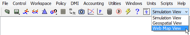
Canvas or Workspace Views
The canvas is the region within the workspace in which models are built and displayed. These canvas is shown when in Full mode, but not shown in Compact mode, as described in Workspace Display Mode.
There are four versions of the canvas which display different Views of the objects and connections.
• The Simulation View displays a schematic of the basin; objects are linked together to form a network.
• The Accounting View (when accounting is enabled) shows a similar schematic, but each object is displayed as a rectangle that contains all the accounts on that object.
• The Geospatial View displays objects at their locations on a static georeferenced background map.
• The Web Map View displays objects on top of a map served from the web. It provides a dynamically zoomed map.
Because of the differences in how the network is displayed in each view, there are different configuration options for each canvas. The following sections describe each canvas and the configuration options.
Note: Each canvas is configured separately. Although the configuration dialogs are the same for the Simulation and Accounting Views, their settings are not shared. Thus, you can configure each independently.
Simulation View
The Simulation View displays a schematic of the basin; objects are represented by icons and are linked together to form a network.
Note: The Simulation View was the original view in RiverWare. As such, most of the screenshots in the RiverWare documentation reference this view when describing models.
Canvas Properties
The canvas configuration dialog is accessed as follows:
• From the menu, select Workspace, then Canvas Properties.
• Right-click the workspace and select Canvas Properties.
The following dialog is shown.
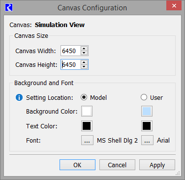
The top portion allows you to change the following attributes of the canvas:
• Canvas Width. Number of pixels
• Canvas Height. Number of pixels
The background and font panel has two controls to select the location of the settings to use:
• Model: Use the model-specific background color, text color, and font shown below. Make any changes to those three settings in the controls below the radio button. The settings will be saved to the model file when it is saved. This is most useful when you share a model and want these three settings to persist among users so the workspace looks the same for all users. This is the default for existing models, saved prior to RiverWare 8.5.
• User: Apply user-specific background color, text color and font. Make any changes to those three settings in the controls below the radio buttons. Note, these changes affect the system registry (saved immediately) and could impact the display of other RiverWare sessions and models the next time you open them. This is most useful when you want these three settings to be tied to a user so that a particular user always sees the same settings. This is the default for new models and is used each time RiverWare opens or the workspace is cleared.
For each location, configure the following settings:
• Background Color.
• Text Color.
• Font including the style and size. This only affects the text on the workspace. See Font and Text Size for the setting to change the application font.
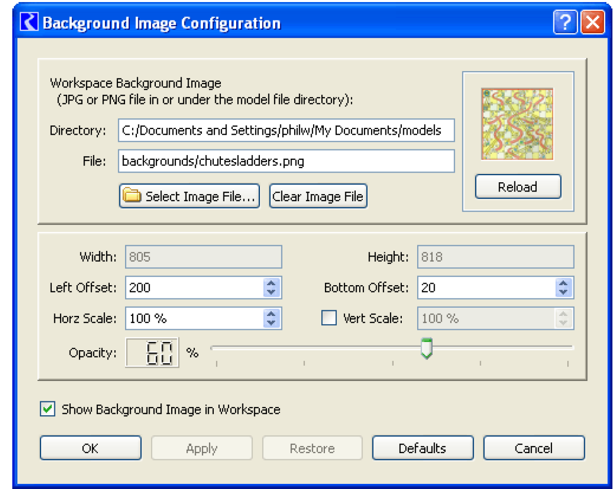
Background Image
The Simulation Workspace supports the ability to show an image loaded from an image file (JPEG or PNG) as the background. The utility is accessed by right-selecting the workspace and choosing Background Image.
The path of the selected image is preserved in the model file (if the model file is saved after configuring the background image). When loading a model with a configured background image file, if the background image file does not actually exist at the recorded path, the model loads without a problem, and the currently-invalid image file path is retained.
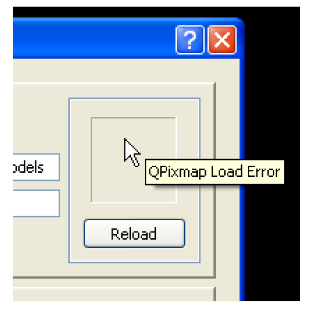
If the selected image file does not represent a valid, supported image file format, the thumbnail (small image preview) will be blank, and the Tooltip on the thumbnail will indicate an error. Figure 2.14 illustrates.
Figure 2.14
Configurable background image properties include the following:
• The image file path (to a JPG or PNG image file).
• The left offset of the image—number of pixels from the left side of the workspace.
• The bottom offset of the image—the number of pixels from the bottom of the workspace.
• The horizontal scale. (100% represents full image scale).
• An optionally independent vertical scale. (100% represents full image scale). If an independent vertical scale is not specified, the configured horizontal scale is used also for the vertical dimension.
• An opacity factor, as a percentage. Zero percent is completely transparent (invisible). 100% is complete opacity, which generally is too opaque unless the actual image is already faded.
• A toggle indicating whether the background image should actually be shown. This has the same state as the similar toggle in the workspace context menu.
A typical use of a background image is a map. This works well if you can reasonably position the icons at approximate positions and/or you do not have or wish to use geospatial coordinate data. But, georeferencing is available on the Geospatial View; see Geospatial View for details. Or show objects on a dynamic map on the Web Map View; see Web Map View for details.
Figure 2.15
Accounting View
If Accounting is enabled, the accounting network is displayed in the Accounting View, and can be selected by the option menu on the toolbar. The accounting view provides a representation of the physical objects, as well as the accounts on those objects where the network can be displayed without occluding or modifying the original physical network.
General configuration of the accounting view is identical to the Simulation View. See Canvas Properties for details.
Note: The settings are independent, not shared.
See Accounting Network in Accounting for details on the Workspace Accounting View.
Geospatial View
The Geospatial View of the workspace provides a spatially coherent display of the modeled basin by associating a map projection and its Cartesian coordinate system with the view. Locate objects and a static background map image in this coordinate system, allowing RiverWare to display a schematic view of the modeled basin overlaid in registry with the map. That is, RiverWare objects are displayed at their location on the map. By providing an intuitive and information-rich view of a basin, the Geospatial view complements the Simulation and Accounting views of the workspace.
Following are key features of the Geospatial View.
• The Geospatial canvas has an associated map projection and location (rectangular extent) within the projection’s coordinate system.
• A map image with a known location in the coordinate system can be displayed in the background layer of the view.
• Images can be georeferenced interactively or automatically via metadata contained within the image file or an accompanying world file.
• The background image (map) can be changed to another with the same projection without requiring any change to the spatial locations (geospatial view coordinates) of the objects.
• Objects are georeferenced (given spatial coordinates) and displayed at that location.
• A distinction is made between an object’s display and actual spatial coordinates.
• Object coordinates can be shared between models and external GIS applications.
• Additional control over the schematic view is provided including sizing and labeling of the icons.
• The coordinates of the cursor in the map projection are continuously presented in the status bar. When available, geographic coordinates (lat/long) are displayed as well.
Introduction to GIS Concepts
Graphical information systems (GISs) support storage, analysis, and display of spatial data. This section introduces some basic GIS terminology and concepts which are relevant to the Geospatial View.
Locations on the spherical earth are most often represented as a pair of coordinates representing latitude and longitude. For some applications, a third coordinate representing an elevation relative to mean sea level is also used. To display a part of the curved surface of the earth on a flat surface necessarily requires a projection, and GIS systems typically represent flat display locations as Cartesian coordinates in a plane onto which the surface of the globe has been projected.
Several standards have been developed to provide agreed-upon coordinate systems for a given area. These standard coordinate systems define a set of map projections which together cover the target area. One common coordinate system which covers the globe is the Universal Transverse Mercator (UTM) coordinate system. This system defines a projection for the northern and southern areas of each of 60 longitudinal zones spanning the globe. For example, in the projection UTM Zone 11 North, the coordinates eastings = 397,800 m, northings = 4,922,900 m, corresponds to a location in central Oregon, USA.
Another standard coordinate system is the State Plane coordinate system which defines a set of projections for the United States. In this system, each state is divided into one or more zones, so a location is specified by a state, zone designation, and x, y coordinates.
Note: A standard coordinate system defines a mathematical coordinate system corresponding to each projection of a set of projections; when these two uses of the term coordinate system would be confusing, we use the term to refer to the standard, and use the term projection or map projection for the component (mathematical) coordinate systems.
Coordinates, whether they be geographic (latitude and longitude) or correspond to a map projection, are specific to a datum. A datum is a reference surface and surveyed coordinates for a set of actual points and lines. Examples of common datums include the North American Datum of 1983 (NAD83) and the World Geodetic System of 1984 (WGS84).
The Geospatial View has a map projection associated with it, and everything displayed in that view (e.g., object icons, background image) needs to be displayed in that projection. Because RiverWare assumes that a single projection is shared between the Geospatial View, the object coordinates, and the map, RiverWare does not need to know the mathematical details of that projection. However, if these details are provided to RiverWare (typically by providing a background image which contains metadata describing the image’s projection), then RiverWare can translate projected coordinates to geographic coordinates, and display these coordinates where appropriate.
Object Coordinates
To support the Geospatial View of the workspace, RiverWare associates coordinates in the view’s projected coordinates system with each object on the workspace. To provide more flexibility for the user, RiverWare supports both Actual and Display spatial coordinates. Actual coordinates are the static coordinates of the object which may come from other sources. The display coordinates are the location where the object is shown on the geospatial view. Often the display coordinates differ from the actual coordinates because the object was moved slightly for less icon clustering or better display.
When an object is created, it is placed at the point of creation in the current view and given locations in the other three views based on its location in the current view. Objects can be moved in any view, and in the Geospatial View this will change the display spatial coordinates. This view also provides the following additional mechanisms to edit or specify spatial coordinates:
• The Object Coordinate Manager dialog displays spatial coordinates for all objects in a single dialog. This dialog supports editing of individual values as well as cut/paste/copy (see section below for more details). This also provide a mechanism to facilitate reconciliation of an object’s actual and display spatial coordinates.
• Import the Actual Coordinates from an ESRI shape file.
Following is a description of the Object Coordinate Manager Dialog which is used to edit/view object coordinates. The Object Coordinate Manager is non-modal and accessed by right-selecting the main workspace (in the Geospatial View) and then selecting Object Coordinates.
The Object Coordinate Manager has tabs for both the Web Map View and Geospatial View. Below is a description of the Geospatial coordinates. See Object Coordinates - Web Map View for information on the Web Map View tab. Note the coordinates are separate for the two views.
The Object Coordinate Manager dialog displays both the display and actual spatial coordinates for all workspace objects. This dialog supports editing of individual fields as well as cut/paste/copy. For each object, both the display and actual spatial coordinates are displayed.
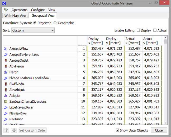
Following are operations that you can perform through the dialog.
• Select Coordinate system. Coordinates are displayed for either the projected or geographic coordinate system. If the canvas has not been configured with full projection information, then RiverWare can not convert to geographic coordinates and this option is disabled.
• Sort. Objects in the table can be sorted using the Sort menu. There are options to sort by Object Type, Object Name, Display X or Y, Actual X or Y, Custom and Custom from Workspace. To use the Custom sort, highlight one or more objects and use the blue up and down arrows to sort the objects. The Custom from Workspace sort option is defined on the workspace Object List; see Simulation Object List.
• Editing. Values in the dialog are only editable when the appropriate Enable Editing toggle is selected. Then, double-click a value and type in a new number.
• Show Data Objects. The Show Data Objects toggle allows you to specify whether you wish to see data objects.
• Show on Workspace. Select one or more objects, then right-click and select Show on Workspace to highlight and select the objects on the workspace.
• Copy Display/Actual Coordinates to the other. The Operations menu has options to Copy Display Coordinates to Actual Coordinates and Copy Actual Coordinates to Display Coordinates. This allows you to move coordinates easily between the display and actual.
Note: These operations copy all values in the column, not the selected ones. When you do this operation, it may overwrite data. Thus, a warning dialog is provided for you to confirm or cancel the operation.
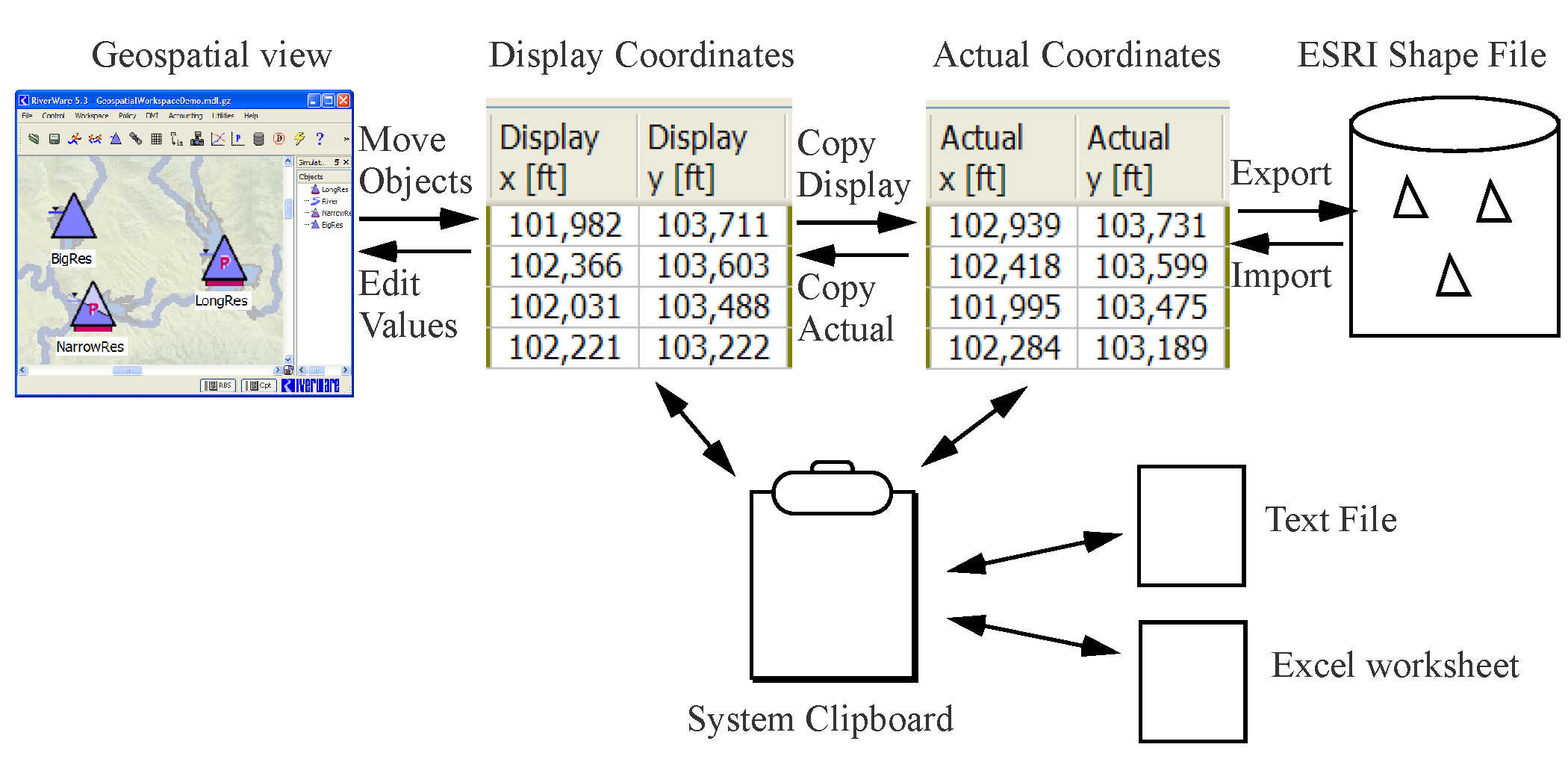
• Export Copy/Import Paste Values. You can copy or paste any values to or from the system clipboard and then to or from external text or Excel files or back to this dialog. This gives you a lot of flexibility in how you move data.
Note: When you copy and paste values, it is operating on the selected values in the sort order as it is displayed. There is also an Export Copy with the Object Names option to also export the RiverWare object name. These operations are available from the right-click context menu.
• Importing/Exporting Coordinates. Import and export spatial coordinates through the ESRI shape file format. In this context, the shape file format is a collection of three files with different suffixes:
– .shp - objects represented as points.
– .shx - indices into .shp file
– .dbf - object attributes (initially object name and object type)
RiverWare supports export of the spatial coordinates of all or selected objects. When coordinates are imported, the user will be warned that the existing coordinates will be overwritten and notified when coordinates for unknown objects are encountered.
Note: Both export and import use the projected coordinate system.
Figure 2.16 illustrates the possible movement of coordinate data within RiverWare.
Note: Any operation using the system clipboard involves a Copy, Cut, and Paste, which involves Export Copy and Import Paste within RiverWare.
Figure 2.16 Data operations in the Object Coordinate Manager dialog
Getting Started With the Geospatial View
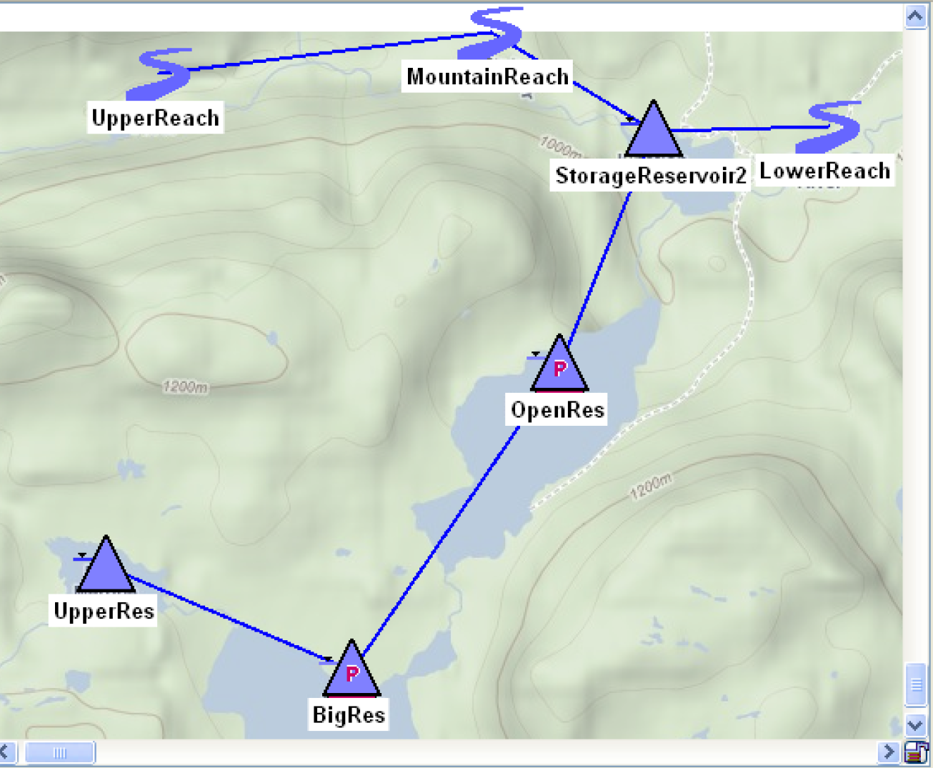
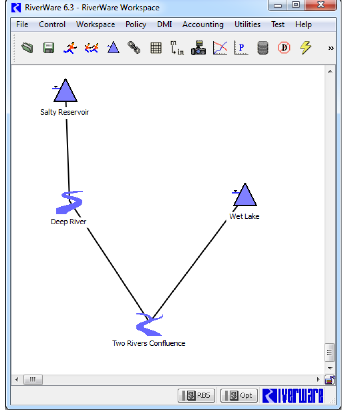
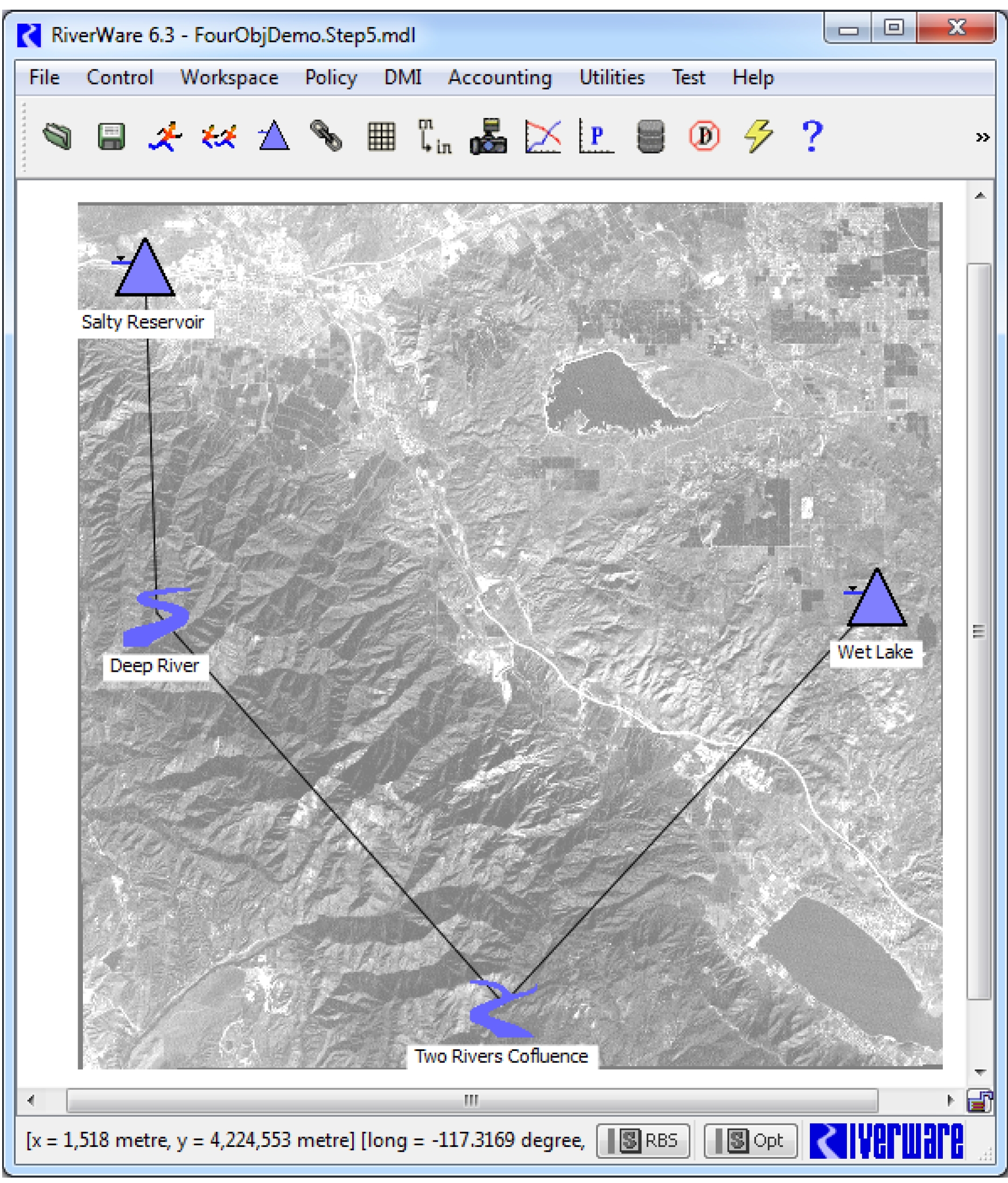
This section describes how you might begin to use the Geospatial View with an existing model which to this point has made use of only the Simulation and/or Accounting Views. Figure 2.17 shows the workspace Simulation View for the model we will be using to illustrate this process.
Figure 2.17 Simulation view of example model
1. Acquire a map of the basin.
As discussed above, the Geospatial View is most useful when you have a basin map with projection information. Such maps can be exported from a GIS application or acquired from a map provider. For example, you can download maps for the United States in a variety of formats from the USGS National Map site:
2. Switch to the Geospatial View.
Initially the positions of the objects in this view will be based on their original placement in another view. Also, at this point, the canvas will have a default configuration and the object coordinates in the default coordinate system (which equates one unit of distance with one display pixel) will likely be orders of magnitude off of their true coordinates in any actual coordinate system. In our example, the southernmost reservoir (Salty Reservoir) is at the northernmost position, and object coordinates are in the range 100–400.
3. Load the map.
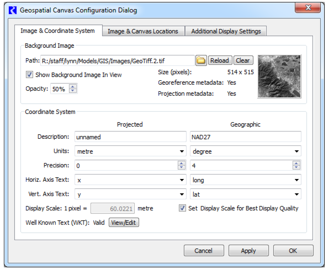
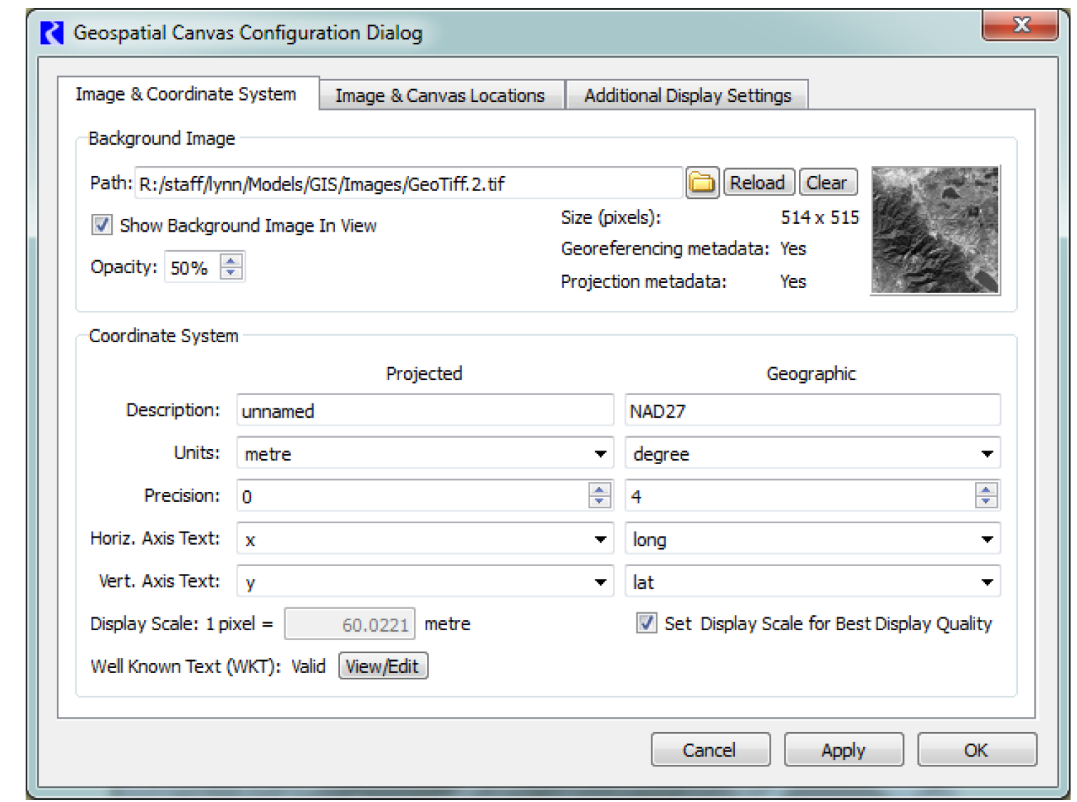
Continuing with our example, open the Geospatial Canvas Configuration dialog and select a GeoTIFF image.
Figure 2.18 Geospatial Canvas Configuration dialog for sample model
Note: There are many supported formats but common ones include GeoTIFF, JPG2000, and MrSID.
As illustrated in Figure 2.19, this is a 514 x 515 pixel image with projection metadata. While the projected coordinate system is not named in the metadata, the geographic coordinate system (datum) on which the projection is based, is NAD27.
Figure 2.19 Geospatial Canvas Configuration dialog for sample model
4. Adjust the Canvas.
By selecting the Image & Canvas Locations tab, we see the location of the image in the projected coordinate system, and we can adjust the canvas size if necessary. By default the canvas is automatically sized to be slightly bigger than the image, which works well for this model.
5. Apply changes.
At this point you have established the basics of the configuration and can apply your changes by selecting OK. Since the default object coordinates are in the hundreds but the image rectangle y coordinates are in the 4000 km range, the objects are not on the canvas as we it is newly configured. Figure 2.20 illustrates the Geospatial View after applying our changes and letting RiverWare automatically place the objects on the canvas.
Note: The status text in the lower left corner of the dialog now shows the location of the cursor coordinates in both the projected and geographic coordinate systems.
Figure 2.20 Geospatial Canvas after importing image
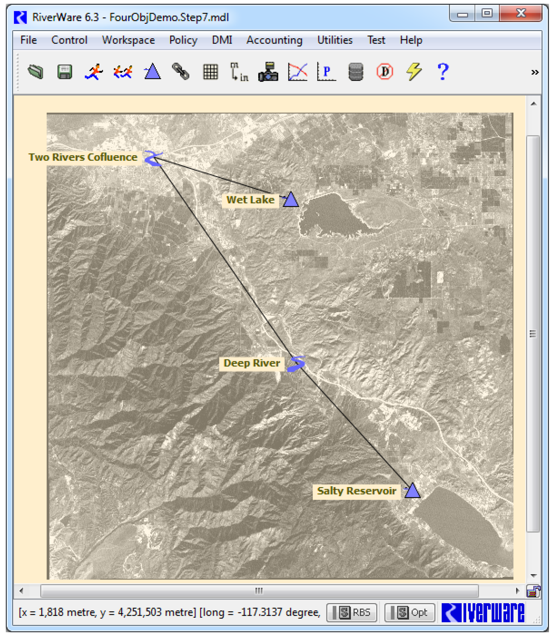
6. Position the objects.
All the objects are on the canvas, but they are not at their true locations. If you knew their coordinates in the projected coordinate system, you could use the Object Coordinate Manager to place them, but for most purposes, placing them by hand in the workspace is adequate. Figure 2.21 shows the workspace after placing the objects at their approximate locations on the map.
Figure 2.21 Geospatial Canvas after moving objects

7. Refine the Configuration.
For this small, low resolution image, the RiverWare icons tend to obscure the map. To improve the display, you can return to the canvas configuration dialog and adjust controls in the Additional Display Settings tab. Figure 2.22 shows the workspace after tinkering with the background color, font, and label orientation, and then adjusting the icon positions further.
Figure 2.22 Geospatial Canvas after adjusting settings
Geospatial Canvas Configuration Dialog
The Geospatial View is most useful when a basin map exists which can be located (georeferenced) in a known projection system. If this information is not available, consider using the Simulation View with a background image.
The Geospatial Canvas Configuration Dialog allows you to specify information about your georeferenced image and how it relates to the RiverWare workspace. It is accessed as follows:
• Right-click the geospatial workspace and select Canvas Properties.
• Select Workspace, then Canvas Properties when the Geospatial View is shown.
We will discuss each of the Geospatial Canvas Configuration Dialog tabs in turn.
Image & Coordinate System Tab
This portion of the dialog describes the background image and the projected and geographic coordinate systems associated with that image (and the Geospatial View in general).
Background Image
Image files are specified by full path names with environment variable expansion. Environment variables are specified using the $PATH syntax. If the image changes outside of RiverWare you may need to reload it using the Reload button.
Of the many image formats supported by RiverWare1, the most common are JPEG, PNG, JPEG 2000, GeoTIFF, and MrSID.When an image is loaded, RiverWare checks for the presence of two type of useful metadata:
• Georeference. Location of the image in its projection.
• Projection. Description of the projection in WKT (well known text) format.
If present, these data are used to set appropriate aspects of the configuration. Some image formats support the embedding of these metadata in the image file itself (e.g., GeoTIFF, JPEG 2000, and MrSID), but RiverWare also checks for a co-located file with a suffix indicating that it contains image metadata. For example, RiverWare will look for an associated file in the world file format, a plain text file format developed by ESRI for georeferencing raster map images.
A valid world file contains six lines, each containing a floating point value, denoted here by the letters A to F. These values define an affine transformation from pixel coordinates to projection coordinates in the form:


where:
– x1 = calculated x-coordinate of the projection location
– y1 = calculated y-coordinate of the projection location
– x = column number of a pixel in the image
– y = row number of a pixel in the image
– A = x-scale; dimension of a pixel in map units in x direction
– B, D = rotation terms
– C, F = translation terms; x, y map coordinates of the center of the upper left pixel
– E = negative of y-scale; dimension of a pixel in map units in y direction
For many GIS applications, creating an image with a world file is relatively straightforward. For example, to do this in ArcMap 10.0, select File, then Export Map, then select the Write World File checkbox in the dialog. On the other hand, when this is not possible, the world file format is simple enough that it can be created by hand with a text editor.
The Geospatial View currently supports only images with unrotated, square pixels, thus not all map images can be displayed as background images. If metadata indicate that these assumptions are violated, RiverWare will notify the user at image load time.
Following are additional controls and information contained in this section of the dialog:
• Checkbox indicating whether to Show Background Image in View.
• Integer indicating the percent Opacity with which to display the image
• Labels indicating the presence or absence of georeference and projection image metadata.
Coordinate System
This panel displays information about the projected and geographic coordinate systems associated with the Geospatial View.
• Description. Textual description of the coordinate system. This could include a technical description of the coordinate system such as “UTM NAD83 Zone 11N”, but RiverWare will not make any assumptions about the description contents.
• Units. Text describing the units of the coordinate system. These are not limited to the units supported for slot values because these are used for display purposes only.
• Precision. Number of digits to the right of the decimal point with which to display coordinates.
• Horiz. Axis. Label associated with the horizontal dimension of the coordinate system. For the projected coordinate system, this is usually “x” or “Easting” but you can also select <custom> and enter your own text. For geographic coordinate systems, this is usually “long” or “longitude”.
• Vert. Axis. Label associated with the vertical dimension of the coordinate system. It is usually “y” or “Nothing” but you can also select <custom> and enter your own text.
• Display Scale. Projection units per pixel used for displaying the canvas on the screen at a zoom factor of 100%. This setting relates the projection to the screen display of the canvas. When the Set Display Scale for Best Quality Display box is checked, RiverWare sets this automatically, usually using the display scale which leads one pixel in the background image to be displayed as one pixel on the screen.
Note: RiverWare uses a single display scale for both vertical and horizontal dimensions.
• Well Known Text (WKT). Indicates whether full projection information is available in the WKT format and allows this text to be view and edited. Typically this description will be set automatically from image metadata, but if the image does not contain this information, it can be provided interactively.
You can either set these fields interactively or, if the appropriate image projection metadata is present, RiverWare will set them automatically.
Note: If the fields are set automatically, it is possible to override the values set from metadata, but they will be reset if the image (and metadata) is reloaded. A preferable approach would be to correct the metadata to contain the desired information.
The geographic coordinate system portion of this panel is only relevant when full projection information is present, typically part of the projection metadata. When this information is not present, this portion of the panel is disabled.
Image & Canvas Locations Tab
This panels displays information about the locations of the background image and canvas in the projected coordinate system.
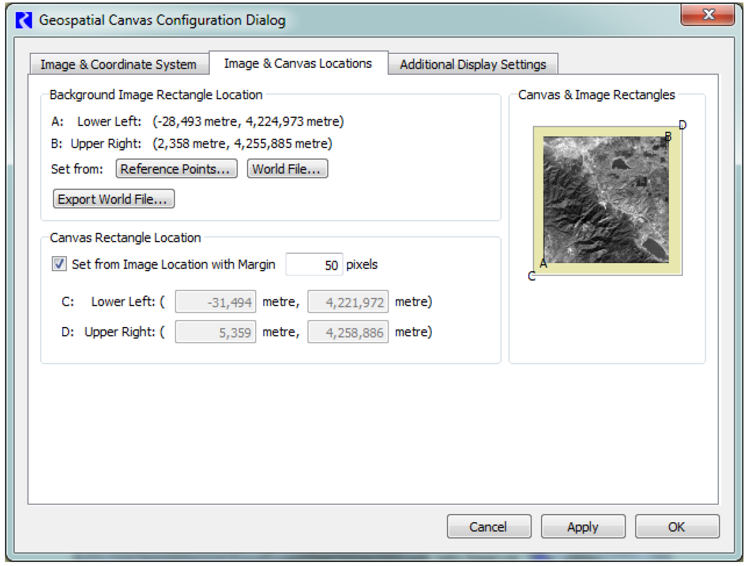
Background Image Rectangle Location
To display the background image at the proper location on the canvas, RiverWare needs to know its location in the projected coordinate system (i.e., the image must be georeferenced). There are two alternatives for providing this information if RiverWare did find it when the image was loaded. One is to select the Set from: World File button. RiverWare will then present a file chooser dialog for specifying the world file containing the image’s georeferencing information. This option is appropriate when an appropriate world file exists, but it is either not co-located with the image or has an unusual name that prevents RiverWare from discovering it.
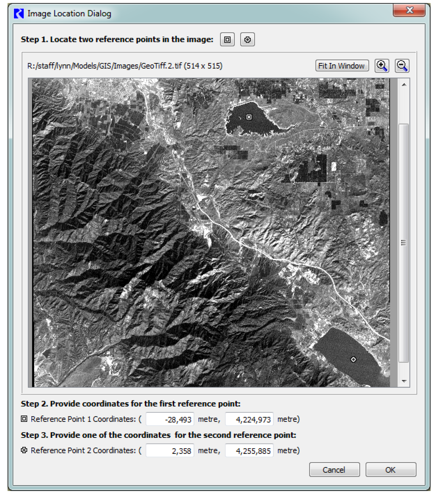
If no metadata is available, then another option is to provide coordinates for two specific locations in the map, in which case RiverWare will use these reference point coordinates to compute projection coordinates for the full image. To provide this information to RiverWare, select the Set from: Reference Points button. This opens the Image Location Dialog which displays a view of your image. For this utility, a reference point is a location for which you know the coordinates and you can locate in the image. Only 2 reference points are needed to locate the image in the projection coordinate system.
As shown in Figure 2.23, you perform the following steps.
1. Locate a reference points in the image. Use the zooming tools to get as close as possible to the first reference location. Select the  button and then select the image to locate the first reference point one. Zoom/Scroll to the second reference location. Select the second button
  and select the image to locate the second reference point.
button and then select the image to locate the first reference point one. Zoom/Scroll to the second reference location. Select the second button and select the image to locate the second reference point. 2. For the first reference point corresponding to enter the coordinates in the dialog.
enter the coordinates in the dialog.3. For the second reference point corresponding to  enter either the x or y coordinate; the other coordinate will be computed by RiverWare.
enter either the x or y coordinate; the other coordinate will be computed by RiverWare. 4. Click OK to confirm the entry and close the dialog.
If you have set the background image rectangle location interactively, you can export the corresponding georeferencing information by selecting the Export World File button. RiverWare will allow you to select a file name and write the background image’s georeferencing information to that file in the world file format. This file can then be used to automatically register the image within other RiverWare models or with any application that can supports the world file format.
Figure 2.23 Geospatial view Image Location dialog
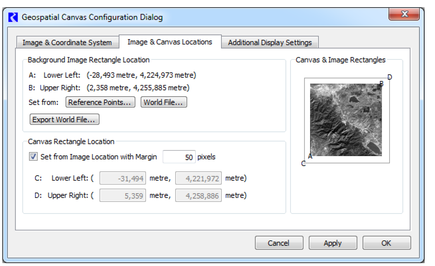
Canvas Rectangle Location
In the Canvas Rectangle Location area, you specify where the canvas rectangle lies in the projection’s coordinate system, by giving the coordinates of the lower left and upper right corners of that rectangle. Checking the Set from Background Image withe Margin checkbox will cause RiverWare to automatically compute the canvas location to be that of the Background Image with an optional margin added to each side. Clearing this box allows you to interactively enter three coordinates of the canvas location (the remaining coordinate will be computed by RiverWare based on the other three). Care should be taken here to enter a canvas location that includes that of the image.
Canvas and Image Rectangles
This panel provides a high-level view of the canvas and image rectangles, drawn as rectangles whose size and relationship to each other matches that defined in the Background Image Rectangle Location and Canvas Rectangle Location panels. The locations of each coordinate (A, B, C, and D) are shown in the thumbnail.
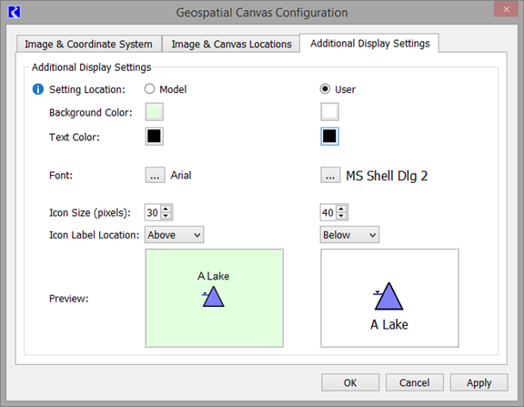
Additional Display Settings Tab
In this tab, you can specify additional display settings for the geospatial workspace.
The background and font panel has two controls to select the location of the settings to use:
• Model: Use the model-specific settings shown below. Make any changes to the settings in the controls below the radio button. The settings will be saved to the model file when it is saved. This is most useful when you share a model and want these settings to persist among users so the workspace looks the same for all users. This is the default for existing models, saved prior to RiverWare 8.5.
• User: Apply user-specific background color, text color and font. Make any changes to those settings in the controls below the radio buttons. Note, these changes affect the system registry (saved immediately) and could impact the display of other RiverWare sessions and models the next time you open them. This is most useful when you want these settings to be tied to a user so that a particular user always sees the same settings. This is the default for new models and is used each time RiverWare opens or the workspace is cleared.
For each setting location, select from:
• Background Color. Select the button to bring up a color chooser.
• Text Color. Select a color for the object label text.
• Font. Provide a font and size for the label text.
• Icon Size (pixels). Enter a value for the RiverWare icon size at 100% zoom factor.
Note: The standard size is 40 pixels. Currently, this setting is global for the geospatial canvas. In the future, this may be changed to a per-object setting.
• Icon Label Location. Select the location of the label: below, above, left, right of the object.
Note: No Label is an option. Currently, this setting is global for the geospatial canvas. In the future, this may be changed to a per-object setting.
All selections in this frame are applied to the sample reservoir icon immediately, but are applied to your workspace when the OK or Apply button is selected.
Applying Configuration Changes
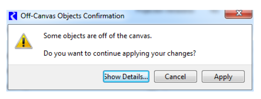
When you are satisfied with the configuration and would like to apply it to the Geospatial View, select OK or Apply at the bottom of the dialog. This will apply changes from all tabs of the dialog (OK will also close the dialog). If the current spatial coordinates of one or more object do not fall within the configured canvas boundaries, you will be prompted with the warning dialog shown. A detailed explanation can be shown, basically explaining that RiverWare expects all objects to be displayed on the canvas, and that continuing the apply operation will cause RiverWare to automatically reposition those objects so that they are on the canvas. This is a reasonable thing to do if this is the first time an image and coordinate system information has been configured for this view. Once the new configuration has been applied the Geospatial View, you can then refine the positions of the object (by direct manipulation with the workspace or using the Object Coordinate Manager, described below). On the other hand, the objects could have correct coordinates for the coordinates system but are off of the canvas due to unintended changes to the canvas location, in which case you should cancel the apply operation and correct any problems.
Following are some strategies for dealing with overlapping icons which is sometimes called icon clustering.
• Use smaller icons and place labels to one side or the other.
• Give clustered objects display spatial coordinates that allow for a clear display, deviating somewhat from their actual coordinates as necessary.
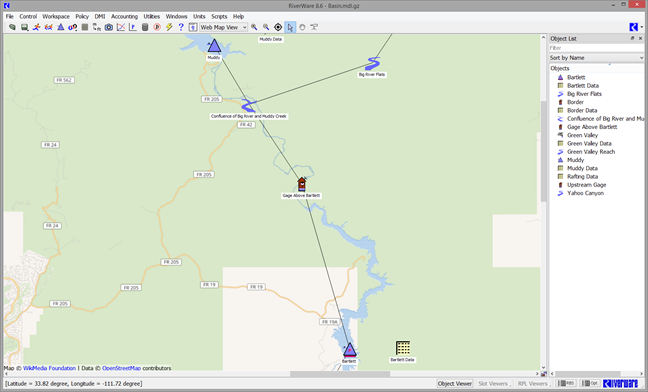
Web Map View
The Web Map View of the workspace provides a spatially coherent display of the modeled basin by displaying objects on top of a dynamic map provided from the Open Street Maps web service.
In this section we first give an overview of the Web Map View and the configuration options. Then we provide a step by step guide on setting up the web map view in Getting Started with the Web Map View.
Tip: When first setting up the Web Map View, please follow the steps in Getting Started with the Web Map View.
A sample configured web map view is shown.
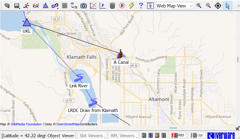
The following are key features of the Web Map View.
• The Web Map View shows a background map provided by the Open Street Maps web service. As you zoom in, the map’s level of detail increases. As you zoom out, the level of detail decreases.
• The Web Map View requires an Internet connection, although once the map tiles have been cached, they will be available for use without a connection.
• Only one type of map is supported. It shows streets, land use, and major water ways. Additional map types may be offered in the future.
• Specify the map extents and home location using a graphical editor.
• Specify the map’s 100% zoom level and see the resulting canvas dimensions
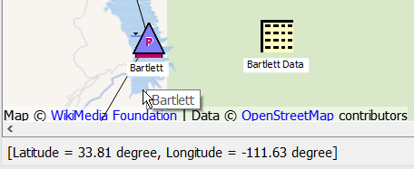
• The Web Map View shows Latitude and Longitude for the coordinates and objects.
• Export and import object coordinates using a shape file.
• Additional control over the schematic view is provided including sizing and labeling of the icons.
• A Home button is provided on the tool bar to get back to one defined location.
• The in-view locator is available but the map is not shown in that view. The Locator Window is not supported for the Web Map View.
Accessing the Web Map View
To access the Web Map View, use the menu:
Canvas Configuration and Properties
The canvas configuration is automatically opened the first time the Web Map View is accessed. It can also be accessed as follows:
• From the menu, select Workspace, then Canvas Properties.
• Right-click the workspace and select Canvas Properties.
The following dialog is shown.
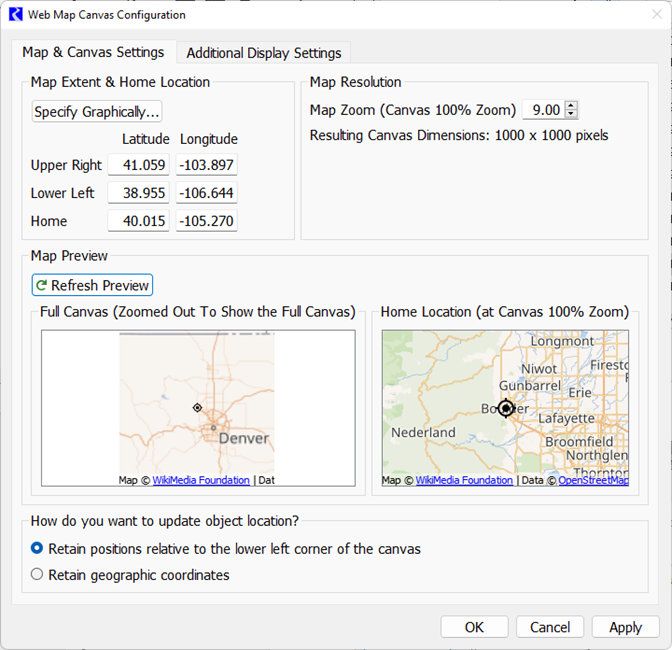
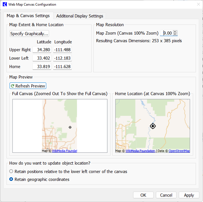
Figure 2.24 Screenshot of the Web Map Canvas Configuration
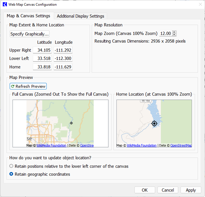
Map & Canvas Settings
The configuration dialog allows you to change the following attributes of the canvas. The first step is to specify the bounds to use for the workspace web map. Either manually specify the coordinates as described in the next section or graphically select your bounds from a web map as described in Map Extent & Home Location Dialog - Graphically Specify Coordinates.
Map Extent & Home Location Panel - Manually Enter Coordinates
If you want to type in the coordinates, enter:
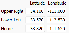
• Upper Right Latitude and Longitude: specify the geographic coordinates of the upper right corner of the view.
• Lower Left Latitude and Longitude: specify the geographic coordinates of the lower left corner of the view.
• Home location: Enter the Latitude and Longitude of the home location. When the Home button on the workspace, shown below, is selected, the view is centered on this Latitude and Longitude, at the current zoom level. This home location is also shown in the two preview maps.

Map Extent & Home Location Dialog - Graphically Specify Coordinates
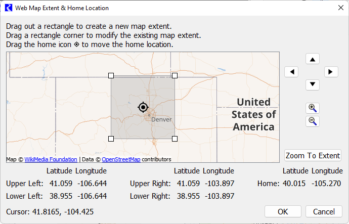
Use the 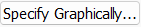 button to open the Web Map Extent and Home Location dialog:
button to open the Web Map Extent and Home Location dialog:Figure 2.25 Screenshot of the Web Map Extent and Home Location Dialog
This dialog shows an unbounded web map and the current canvas bounds represented by a rectangle and the Home location icon within the rectangle. To specify the extents, use the following steps:
1. If necessary, use the panning and zooming tools, shown below, to find the correct area of the world. The middle mouse button will also pan the map when clicked.
2. Drag out a new rectangle on the map to define the boundaries.
3. Drag the corners of the rectangle to modify the existing corners.
4. Drag the Home Location icon to move it as desired.
The resulting Latitude and Longitudes are shown at the bottom of the dialog.
When finished, select OK and the dimensions will be copied to the Web Map Canvas Configuration.
Map Resolution
• Map Zoom (Canvas 100% Zoom) - Specify the relative zoom level that corresponds to 100% zoom on the workspace. The valid entries are 2 to 15. A value of 2 represents continent-level maps. 15 represents street-level maps.
• Resulting Canvas Dimensions. The height and width in canvas pixels is computed based on the corners and the relative zoom level. The higher the zoom level, the larger the dimensions.
Map Preview
When setting up the map and home location, use the Refresh Preview button to show two maps: Full canvas and Home location at 100% zoom.
How do you want to update object locations?
When you select OK or Apply, any changes to the zoom level or bounding coordinates could result in changes to either where in the view objects are or to the geographic coordinates of the objects. Select from the two choices on how to update object locations:
• Retain positions relative to the lower left corner of the canvas: The objects will be moved to be on the new canvas, if possible, but keeping relative positions. This is most commonly used when first setting up the Web Map View. Technically, for this option, the object canvas coordinates remain the same and the geographic coordinates change.
• Retain geographic coordinate: This assumes the objects are in the correct latitude and longitude and they should retain those locations. The objects will stay in their relative place on the map. This is most commonly used when updating a map after the objects have been placed in the correct location. Technically, for this option, the object geographic coordinates remain the same and the canvas coordinates change.
Additional Display Settings
The Additional Display Settings tab has two controls to select the location of the settings to use:
• Model: Use the model-specific background color, text color, and font shown below. Make any changes to those three settings in the controls below the radio button. The settings will be saved to the model file when it is saved. This is most useful when you share a model and want these three settings to persist among users so the workspace looks the same for all users. This is the default for existing models, saved prior to RiverWare 8.5.
• User: Apply user-specific background color, text color and font. Make any changes to those three settings in the controls below the radio buttons. Note, these changes affect the system registry (saved immediately) and could impact the display of other RiverWare sessions and models the next time you open them. This is most useful when you want these three settings to be tied to a user so that a particular user always sees the same settings. This is the default for new models and is used each time RiverWare opens or the workspace is cleared.
For each location, configure the following settings:
• Background Color.
• Text Color.
• Font including the style and size. This only affects the text on the workspace. See Font and Text Size for the setting to change the application font.
• Icon Size (pixels).
• Icon Label Location.
A preview shows what the object will look like on the workspace.
Object Coordinates - Web Map View
To support the Web Map View of the workspace, RiverWare saves both the canvas coordinates and geographic coordinates for each object on the workspace.
When an object is created, it is placed at the point of creation in the current view and given locations in the other three views based on its location in the current view. This view also provides the following additional mechanisms to edit or specify spatial coordinates:
• The Object Coordinate Manager dialog displays spatial coordinates for all objects in a single dialog. This dialog supports editing of individual values as well as cut/paste/copy (see section below for more details).
• Import / export coordinates from an ESRI shape file.
Following is a description of the Object Coordinate Manager Dialog which is used to edit/view object coordinates. The Object Coordinate Manager is accessed by right-selecting the main workspace (in the Web Map View) and then selecting Object Coordinates.
The Object Coordinate Manager has tabs for both the Web Map View and Geospatial View. Below is a description of the Geospatial coordinates. See Object Coordinates for information on the Geospatial View tab. Note the coordinates are separate for the two views.
Figure 2.26 Screenshot of Object Coordinate Manager
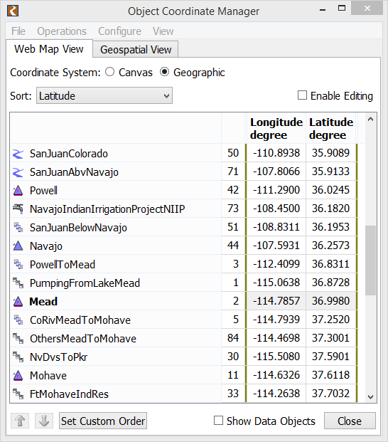
The Object Coordinate Manager dialog displays either canvas coordinates (x, y) or Longitude and Latitude. Select the Enable Editing checkbox to edit the coordinates.
Following are operations that you can perform through the dialog.
• Select Coordinate system. Coordinates are displayed for either the canvas or geographic coordinate system.
• Sort. Objects in the table can be sorted using the Sort menu. There are options to sort by Object Type, Object Name, Display X or Y, Actual X or Y, Custom and Custom from Workspace. To use the Custom sort, highlight one or more objects and use the blue up and down arrows to sort the objects. The Custom from Workspace sort option is defined on the workspace Object List; see Simulation Object List.
• Editing. Values in the dialog are only editable when the appropriate Enable Editing toggle is selected. Then, double-click a value and type in a new number.
• Show Data Objects. The Show Data Objects toggle allows you to specify whether you wish to see data objects.
• Show on Workspace. Select one or more objects, then right-click and select Show on Workspace to highlight and select the objects on the workspace.
• Export Copy/Import Paste Values. You can copy or paste any values to or from the system clipboard and then to or from external text or Excel files or back to this dialog. This gives you a lot of flexibility in how you move data.
Note: When you copy and paste values, it is operating on the selected values in the sort order as it is displayed. There is also an Export Copy with the Object Names option to also export the RiverWare object name. These operations are available from the right-click context menu.
• Importing/Exporting Coordinates. Import and export spatial coordinates through the ESRI shape file format. In this context, the shape file format is a collection of three files with different suffixes:
– .shp - objects represented as points.
– .shx - indices into .shp file
– .dbf - object attributes (initially object name and object type)
RiverWare supports export of the spatial coordinates of all or selected objects. When coordinates are imported, the user will be warned that the existing coordinates will be overwritten and notified when coordinates for unknown objects are encountered.
Note: Both export and import use the geographic coordinate system.
Getting Started with the Web Map View
This section provides a step-by-step approach and recommended tips to set up the Web Map View.
1. Switch to the Web Map View on the workspace using the menu:
Caution: This can take a few seconds to open as RiverWare contacts the server and gets the default maps.
Note: An Internet connection is required for the Web Map View especially during setup of a new basin
2. The Web Map Canvas Configuration dialog opens and is centered on Boulder, Colorado, the home of RiverWare.
Tip: For additional detail on any of these settings, seeCanvas Configuration and Properties.
Now specify the location of your basin. If you know the coordinates, you can type in the upper right and lower left coordinates of your basin, but more likely, you will want to specify these graphically. Let’s use the graphical editor.
3. Select Specify Graphically. The following window opens.
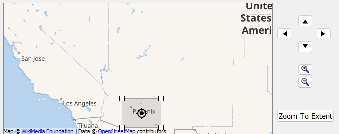
4. Use the controls on the right to zoom and pan to the location of your basin. For this example, we will use a basin in Arizona. So we have panned and zoomed to that area.
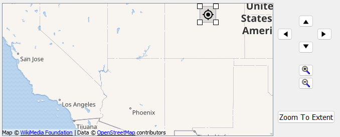
5. Drag out a new rectangle that roughly represents your basin extent. For us, the area is near Phoenix so we drag out a rectangle there.
When we release the mouse button, it moves the extent and home location as shown. The home is set to the center of the rectangle:
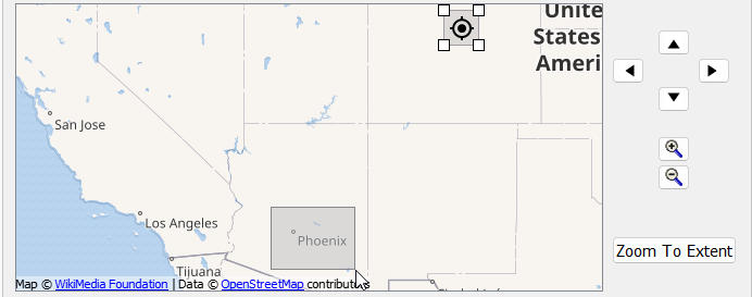
6. Select the Zoom to Extent button.
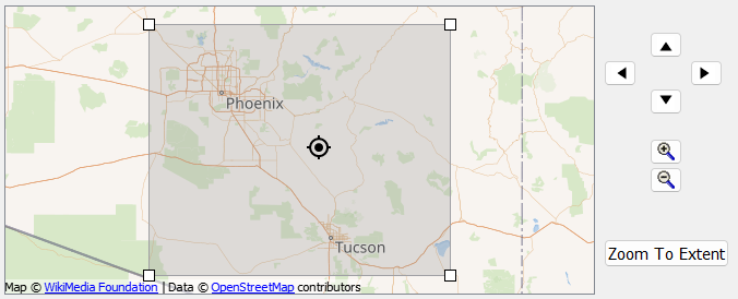
7. Now move the rectangle corner anchors and home icon to refine your basin location. Use the Zoom to Extent and zoom and pan buttons as needed. Here is our result:
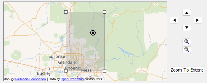
8. Select OK and it shows those coordinates in the Canvas Configuration and the preview is updated:
9. Next specify the 100% Zoom Level - The valid entries are approximately 2 to 15. 2 represents continent-level maps. 15 represents street-level maps. As you change the Map Zoom level, the resulting canvas dimensions change.
The Web Map View zoom levels range from 3% to 400%. The 100% zoom level is the standard zoom level; you will be able to zoom in by a factor of 4 (to 400%) and zoom out to the full extent (5%-20%).
10. Use the Refresh Preview button to see the result of your coordinate entry and zoom level.
We set ours to 12. The result is:
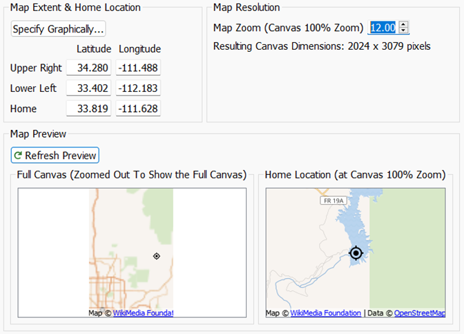
Tip: The preview panels sometimes show extra area when the configuration is first opened. Select Refresh Preview to fix the preview.
11. Iterate steps through 10. until satisfied. This part is a bit of trial and error to get the desired area and 100% zoom level.
12. When first setting up the canvas, you will likely use the “Retain positions relative to the lower left corner of the canvas”. Once you’ve set it up once, you may use the other option “Retain Geographic Coordinates” to keep the objects in their geographic locations on the map.
13. Select Apply
– If you get a message about objects being moved off the canvas, select Cancel and increase the zoom level so your dimensions increase. Select Apply again.
– If you get a message about the canvas being larger than the valid range, select Cancel and decrease the zoom level. Select Apply again.
– If you get a message about the canvas being smaller than the valid range, select Cancel and change your upper right and lower left to be a larger area or increase the zoom level. Select Apply again.
14. Switch to the Additional Display Settings and make any changes as necessary or desired. For smaller basins, you may wish to make the icon size and font size smaller.
15. When finished, select OK.
16. At this point, the objects are likely not in the desired locations. Either drag them to the desired place or import or specify the coordinates using the Object Coordinates - Web Map View.
17. The final product is shown-- the objects are in the correct location and you can zoom in and out on the web map.
Tips on Using the Web Map View
The Web Map View behaves like the Simulation View with the following differences:
• The Locator Window is not supported
• The In-view Locator is supported but no web map is shown. Only the objects are shown.
• The toolbar contains a Home button. Select the button to go to the defined location at the current view. See Home location: Enter the Latitude and Longitude of the home location. When the Home button on the workspace, shown below, is selected, the view is centered on this Latitude and Longitude, at the current zoom level. This home location is also shown in the two preview maps..
to go to the defined location at the current view. See Home location: Enter the Latitude and Longitude of the home location. When the Home button on the workspace, shown below, is selected, the view is centered on this Latitude and Longitude, at the current zoom level. This home location is also shown in the two preview maps..• Modify object locations by moving them on the Web Map View. Alternatively, use the Object Coordinate Manager using the right-click context menu and selecting Object Coordinates.
• The status on the lower left corner of the workspace shows the Latitude and Longitude.
1 RiverWare uses the GDAL open source library to read image files. This library supports over 100 raster data formats, though many of these formats are not suitable for background images because they do not contain color rendering information.
Revised: 01/11/2023