
About Preemptive Linear Goal Programming
This section provides a conceptual overview to the Preemptive Linear Goal Programming solution used by RiverWare Optimization. It begins with brief, general descriptions of linear programming, goal programming and preemptive goal programming. These are followed by some simple examples to illustrate the use of preemptive goal programming to handle conflicting objectives and conflicting constraints.
Linear Programming
The RiverWare Optimization solver uses linear programming at its core. Linear programming is a common optimization approach where linear objective function is maximized or minimized subject to a set of linear constraints.
Maximize 
Subject to:


...

where each x is a variable in the problem. Each c is a numeric coefficient in the objective function. Each a is a numeric coefficient in a constraint. Each b is the numeric right-hand-side value of each constraint. Each constraint can be an “equal-to,” “less-than-or-equal-to,” or “greater-than-or-equal-to” constraint. The objective function and the left-hand-side of every constraint must be a linear combination of one or more variables. Additional general information about linear programming, including approaches for solving a linear program, are covered in any text on the basics of linear programming optimization and thus are not covered here.
In RiverWare, an optimization model ultimately gets formulated as a linear program. The details about that formulation are covered in following sections.
Goal Programming
One limitation of standard linear programming is that all constraints are hard constraints. If there is not a solution that can simultaneously satisfy all constraints, then the problem is infeasible. Also, there is only a single objective function.
Often in water resources contexts, a system will have multiple objectives that need to be traded off against each other. For example, there might be an objective to maximize the value of hydropower generation, but that must also be traded off with environmental objectives and an objective to carry sufficient reserve capacity. If environmental objectives are expressed as constraints (e.g. minimum and maximum flows), cases can result in which the problem becomes infeasible. For example, low inflow inputs can produce a case in which it is not possible to simultaneously satisfy minimum reservoir level constraints and minimum outflow requirements.
One approach to handle the case of conflicting objectives or conflicting constraints is goal programming. In traditional goal programming, a penalty function is applied to any deviation from a constraint value, and the penalties are minimized as part of the objective function. Typically penalty functions are convex. Most often the penalty function is linear, piecewise linear or quadratic because of the available solution mechanisms. For example, some objectives have a term that minimizes the sum of squared violations. In order to combine terms with non-commensurate units in a single objective, the deviations are typically scaled. Additionally the penalty functions and multiple objectives in the objective function might be weighted to express the relative importance of some policies over others. One challenge of this approach is that it can be difficult to interpret the meaning of the weights applied. Also the solution can be sensitive the weights that are used, and it can be difficult to anticipate the effects of modifying weights without significant trial and error.
Rather than combining weighted penalty terms and weighted objectives in a single objective function, RiverWare Optimization uses an alternative form of goal programming referred to as preemptive goal programming, which is described in the following section.
Preemptive Goal Programming
RiverWare Optimization uses a form of goal programming referred to as preemptive goal programming. Constraints and objectives are expressed at distinct priorities. At each priority an optimization problem is solved either to maximize or minimize the stated objective at that priority. If the priority contains constraints, the objective is to maximize the satisfaction of the constraints. (In RiverWare, this derived objective to maximize constraint satisfaction is automatically formulated based on the constraints that the user specifies.) Before moving on to the next priority, the objective value is frozen. This is the equivalent of adding a constraint to the problem that sets the objective function expression equal to the objective value. See Freezing Constraints and Variables for a detailed explanation and example of the concept of freezing. This freezing guarantees that lower priority constraints and objectives will not degrade higher priority constraints and objectives. After the higher priority solutions, there are typically many alternative optima, multiple feasible solutions that would equally maximize the objective function. Any solution for a lower priority must come from the set of alternative optima from the preceding solution. As the solution proceeds through the priorities, the solution space is reduced by the constraints added at each priority. Another way to say this is that the set of alternative optima is reduced, or degrees of freedom are removed from the problem.
The following simple example illustrates the basic concepts of preemptive goal programming, including prioritized objectives, the shrinking solution space, alternative optima and freezing of variables and constraints.
Assume we have two variables, a and b. The problem has only two dimensions. The variables are constrained by the following (hard constraints):


These constraints limit the solution space, as illustrated in Figure 2.1. In other words, they have removed degrees of freedom from the solution.
Figure 2.1
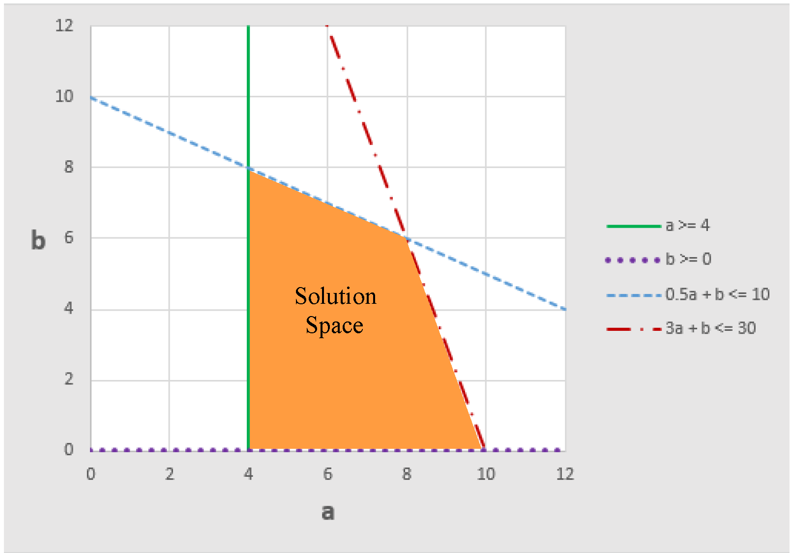
Any feasible solution must be within the orange region (including the edges that bound the region).
The problem has two prioritized objectives.
• Objective 1 (highest priority): Maximize z1 = 3a + b
• Objective 2: (lower priority): Maximize z2 = b
First, we will solve for the highest priority objective, Maximize z1 = 3a + b.
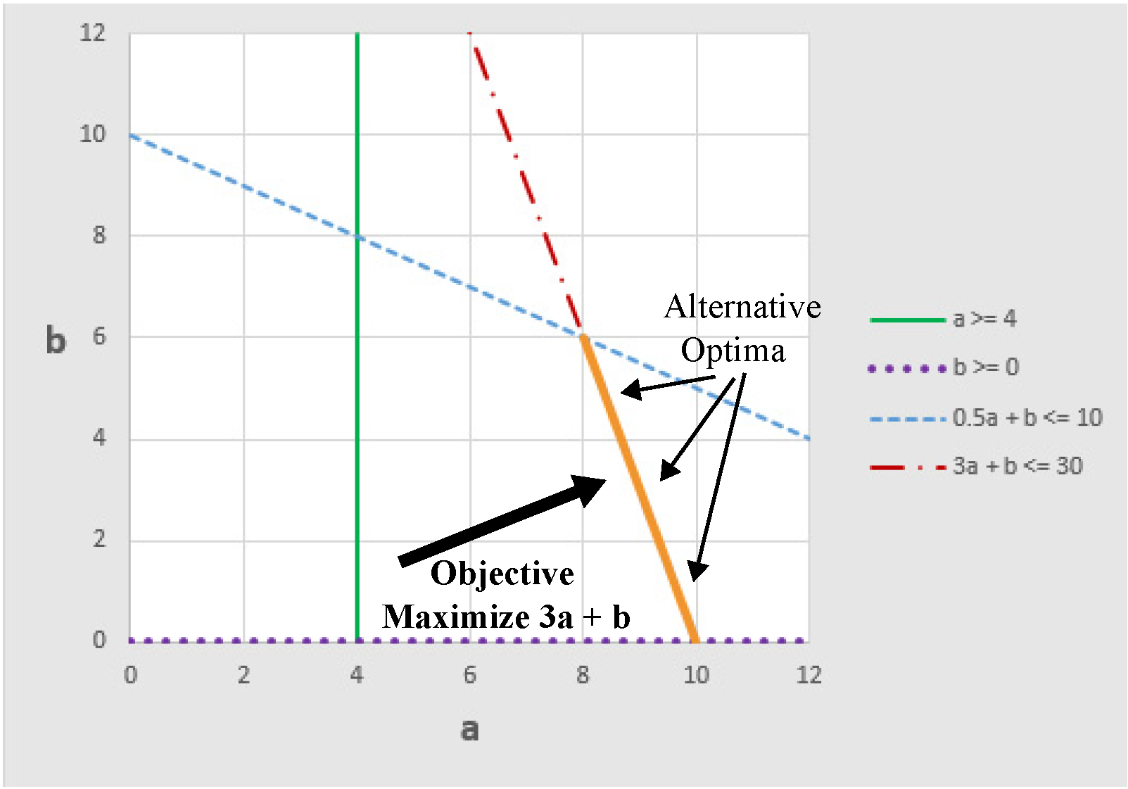
The figure above shows the direction that the objective is pushing the solution. In this case, there are many possible solutions that will equally maximize the objective. Another way to state this is that there are alternative optima. Any point that is on the line 3a + b = 30 with a between 8 and 10 (equivalently, b between 0 and 6) satisfies all constraints and equally maximizes the objective. The alternative optima are illustrated by the orange line segment in the figure above. Given the current set of constraints and objectives we have included in the problem (we have not yet added Objective 2), there is no preference for one point over another from this set of alternative optima. If we increase a, then we must decrease b, but in all cases the objective value, z1, is 30. The simplex method for solving linear programs tends to generate extreme point solutions. In this case it would generate a solution at one of the end points of the line segment.
Now as we move on to Objective 2, we will not degrade the objective value of the higher priority Objective 1. In order to guarantee that Objective 2 does not degrade Objective 1, we will only use the solutions from the set of alternative optima from Objective 1. This is done by freezing the objective value with an “equal-to” constraint:

Note: We have frozen the constraint  by changing it to an “equal to” constraint.
by changing it to an “equal to” constraint.The new constraint reduces the solution space to the orange line segment in the figure above (i.e. remove degrees of freedom).
Now we apply Objective 2: Maximize z2 = b. This is illustrated in the next figure. Once again the large arrow shows the direction that the objective is driving the solution.
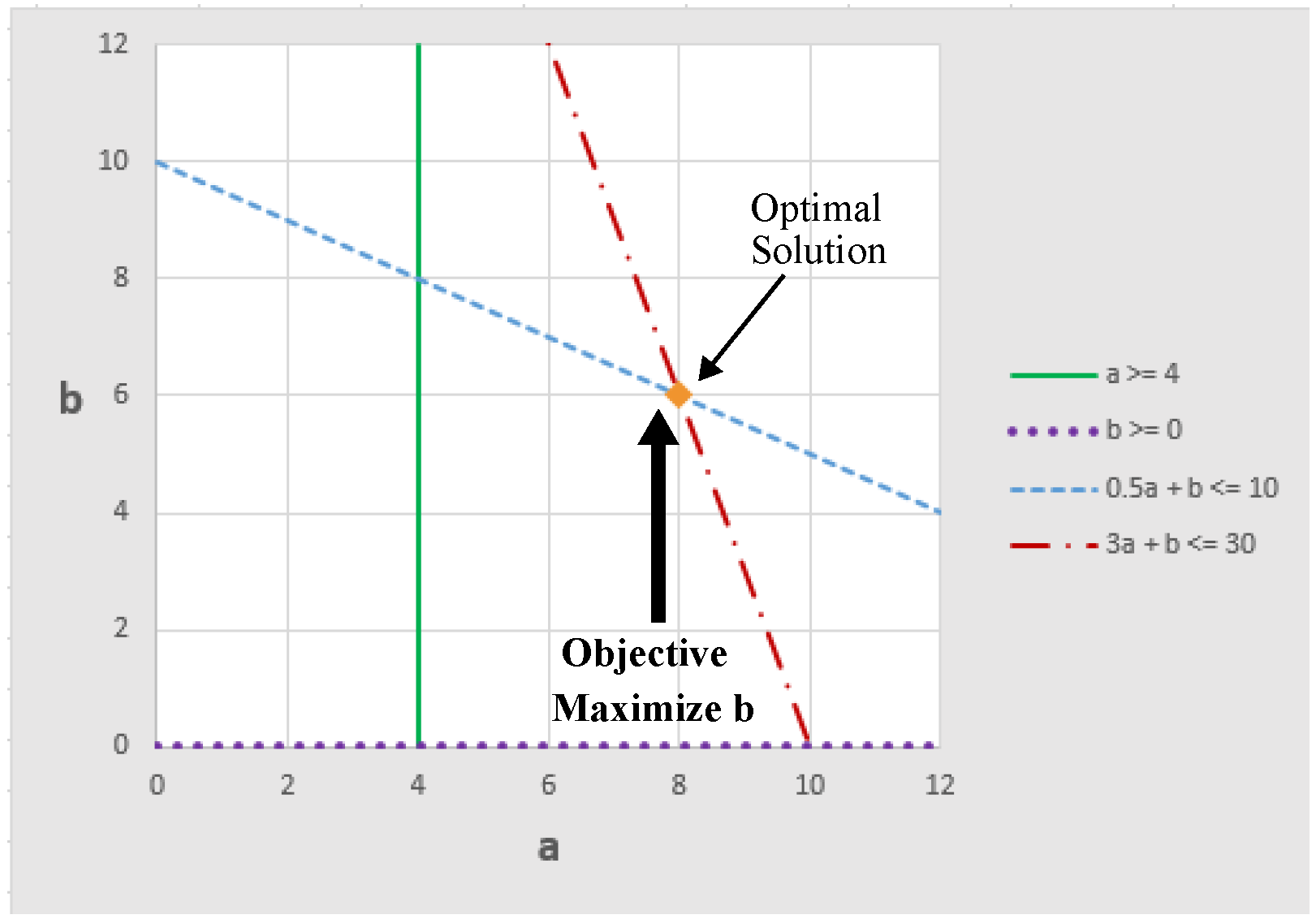
In this case, the objective evaluates to a single optimal solution with the following values for all variables:


All degrees of freedom have been removed from the solution. There are no longer any alternative optima, only a single optimal solution.
Now let’s assume we have the same problem, but we reverse the priorities of the two objectives.
Objective 1 (highest priority): Maximize z1 = b
Objective 2: (lower priority): Maximize z2 = 3a + b
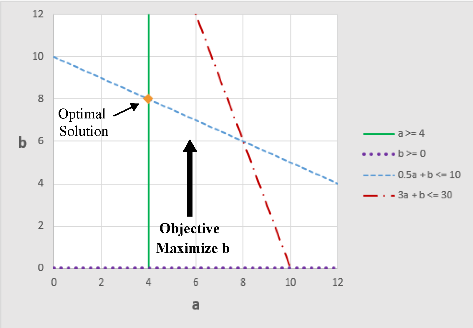
In this case, Objective 1 would remove all degrees of freedom, evaluating to a single optimal solution, as illustrated in Figure 2.2.
Figure 2.2
The objective value gets frozen as.

The constraint  also gets frozen, changing it to an “equal to” constraint.
also gets frozen, changing it to an “equal to” constraint.
In addition the constraint  gets frozen.
gets frozen.
There are no alternative optima, so there are no degrees of freedom left for Objective 2 to affect the solution. The final solution is determined after Objective 1.


Revised: 01/11/2023