
Alternative Routing Coefficients Methods
In the USACE‑SWD flood control routing methods, releases are routed using the Step Response routing method. During extreme large events with overbank flow, the channel routing coefficients are insufficiently accurate to model the routing of water down the reach, i.e., large flows that occupy the overbanks have different travel times. This section outlines the required simulation functionality and proposes a design to add the capability to RiverWare to provide for alternative routing coefficients during high flows, both in the reach simulation and in the flood control release algorithm.
The USACE‑SWD typically uses the Step Response Routing method to route water in RiverWare simulations. There are two separate sets of routing coefficients used, one set for each control point and one set for each reach. The control point routing coefficients are used in the flood control algorithm’s release determination while the reach routing coefficients are used in the simulation to route water. These two routing methods are described below.
One set of routing coefficients for each upstream reservoir resides on the control point Routing Coefficients slot. These coefficients are used only in the flood control algorithm to estimate the effect reservoir releases would have on downstream flooding. In the flood control algorithm water is routed from each upstream reservoir directly to the control point (i.e. reservoir outflow routed to control point) using Equation 2.2.
(2.2) 
The estimated flow at the control point is the sum of the contribution from each upstream reservoir. This equation is only used in the routing in the flood control calculation (i.e. rule function evaluation) and does not actually route water to the control point. These calculations are used by the rule to set reservoir outflows.
The reach is used to route water in the simulation after reservoir outflows have been set. On the reach, the following equation is used to incrementally route water in the reach (i.e. route Inflow plus Local Inflows to Outflow) during the simulation. Step Response routing uses Equation 2.3.
(2.3) 
This equation is used to calculate the current and future outflows (from t = current to t = number of coeffs). All of the C values are calculated outside of the model and for each set of coefficients, the C values sum to 1.0.
To simulate large flows accurately, it is necessary to use alternative routing coefficients only at high flows for both the flood control calculation and the reach simulation. These routing coefficients come into effect when flows are above thresholds. These coefficients are used when the flow is above a threshold in both the flood control algorithm and the reach routing.
Note: It is not necessary to use Step Response Routing on the reaches for simulation/dispatching. You can use any routing method you want. Of course the routing will not match the linear routing used in the flood control algorithm. If you do use a different routing method on the reaches, you will need to still specify routing coefficients on the Control Points. If you wish to use flow based routing coefficients, you will need to select the Variable Step Coefficients method in the Alternative Routing on Subbasin category. This is described below.
User Implementation
To implement the above approach, various methods must be selected.
In the simulation/calibration model, you have the following choices:
• Select the Variable Step Response routing method on the reach. This method adds the alternative coefficients table slot.
• If you wish to not use the Variable Step Response method for simulation/dispatching, select a different routing method, like Modified Puls. But, you must then select Variable Step Coefficients in the Alternative Routing on Subbasin category.
Then, populate the Variable Lag Coefficients table slot with data.
When Flood Control is implemented, a computational subbasin must have the correct method selections. Generally, the same subbasin used for Flood Control should be used for this purpose; see Flood Control for details. This subbasin will contain most, if not all objects in the basin. On this subbasin, select the Compute Aggregate Coefficients method in the Control Point Variable Routing Coefficients category.
Additionally, on each control point downstream of a reach with alternative coefficients, the user must select the Compute Aggregate Coefficients method or Compute Aggregate Coeffs every Timestep method in the Variable Routing Coefficients category. No additional data entry is required on the control point for this method (although the standard Routing Coefficients table are typically input on the control point for the normal flow conditions).
Methods
To enable this approach, the user must select methods on the objects summarized in Table 2.4.
Object | Category | Method | Section in Objects |
|---|---|---|---|
Reach | Routing Method | Variable Step Response | |
Reach | Alternative Routing on Subbasin | Variable Step Coefficients | |
Control Point | Variable Routing Coefficients | Compute Aggregate Coefficients | |
Control Point | Variable Routing Coefficients | Compute Aggregate Coeffs every Timestep | |
Computational Subbasin | Control Point Variable Routing Coefficients | Compute Aggregate Coefficients |
Alternative Routing and Flood Control
The flood control algorithm accesses the correct set of routing coefficients based on the method selection. On a given control point,
• If the Compute Aggregate Coefficients method is selected, the calculated Computed Routing Coefficients will be used. These represent the coefficients determined by the subbasin at the beginning of the timestep. If they were not recalculated (flows did not go above the first threshold), they will contain the same values as the Routing Coefficients slot.
• If the Compute Aggregate Coeffs every Timestep method is selected, the calculated Computed Routing Coefficients will be used. These represent the coefficients determined by the subbasin at the beginning of every timestep.
• If the None method is selected on the control point, the existing Routing Coefficients slot will be used.
Once the set of coefficients are determined, the flood control algorithm proceeds as usual. The algorithm will use the coefficients throughout flood control execution and throughout the forecast period.
Post-run Dispatching
Forecasting and basin lag times result in situations where the last timesteps of the run may not solve correctly if the objects have not solved past the end of the run. To allow objects to solve past the end of the run, you must configure post-run dispatching. Figure 2.5 shows a timeline diagram when post-run dispatching will occur.
Figure 2.5
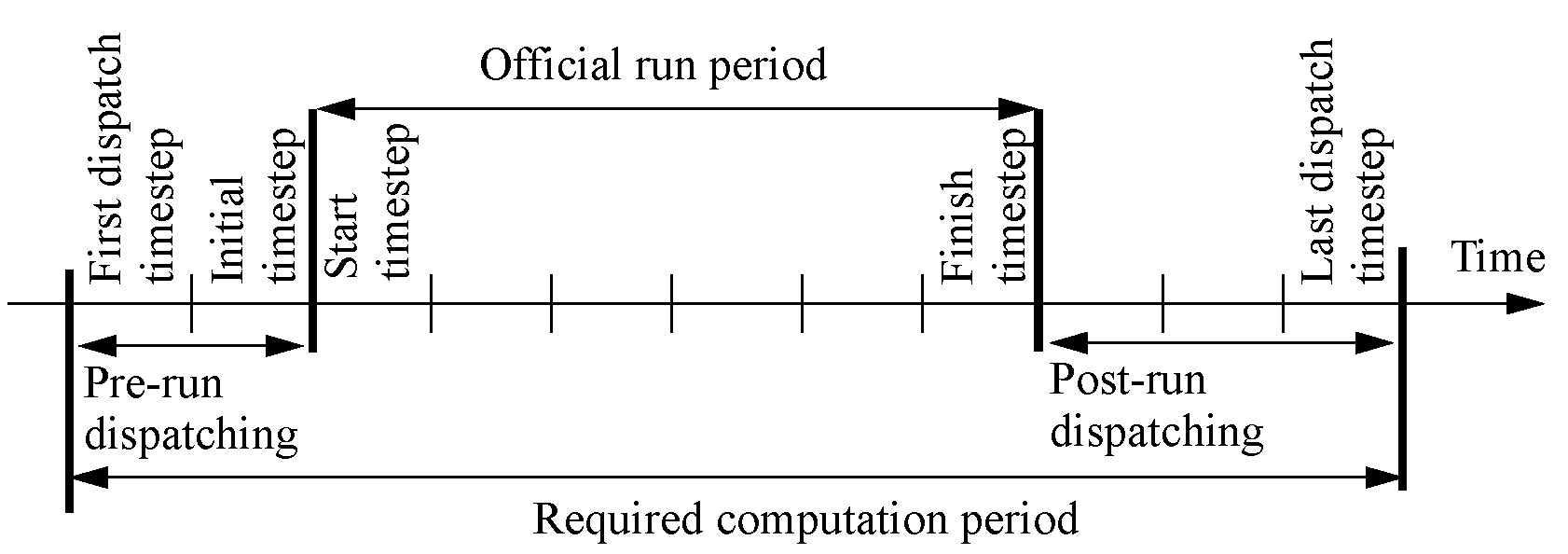
To configure post-run dispatching, set the number of post-run dispatch timesteps equal to the forecast period; see Number of Post-Run Dispatch Timesteps in User Interface for details. For dispatching to occur after the end of the run, certain data must be specified. Following is a description of the required data for post run dispatching
Local Inflow Forecasting Algorithms
The forecasting and disaggregation of cumulative local inflows is done at the beginning of each timestep. The forecasting will be executed at Begin Timestep on the last timestep, but will not occur after that. That is, even though the objects dispatch past the end of the run, no additional forecasting is required. But, local inflow data is required after the end of the run through the Period of Perfect Knowledge. That is, the user only needs to input Cumulative Local Inflows through the run end plus the Period of Perfect Knowledge on each inflow location.
Data Filled for Each Object
Following is data that will be automatically filled in at beginning of run and there is not a valid value. No user interaction is required.
• Reservoir.Diversion
• Reservoir.ReturnFlow
• Reservoir.Precipitation Rate
Data That Must be Input
Following is data that is typically input by the user (input or using a DMI). These will need to be input for post-run timesteps as well. DMIs or rules (RBS or Init) can be configured to quickly set this data.
• Headwater inflows. Gage.Inflow, Control Point.Inflow, Confluence.Inflow 1 or 2 or Reservoir.Inflow, Reach.Inflow. These are typically set to zero.
• Reservoir.Evaporation Rate or Evaporation (defaults to zero if not input)
• Reservoir.Cumulative Hydrologic Inflow and Control Point.Cumulative Local Inflow (or Deterministic Incremental Hydrologic or Local Inflow) See section above for data requirements.
Data Currently Input but Can be Set by Alternative Method Selections
Following is data that is may be input, but with different method selections, the data can be automatically set for all timesteps, including post-run.
• WaterUser.Fractional Return Flow. Select Periodic Fraction method and input a value. Make sure there are no other input values on these slots.
• Reservoir.Seepage. Select Single Value Seepage. Otherwise, seepage defaults to zero if not input.
Revised: 06/04/2022