
Flood Control
The Flood Control methods calculate a flood control release for the current simulation day. The two flood control methods—Operating Level Balancing and Phase Balancing—are invoked from a predefined rules function, and their results are returned to the calling rule.
Note: See Flood Control in USACE‑SWD Modeling Techniques for details on this approach for USACE-SWD methods. The flood control methods (other than None) use forecast data (storage, inflows, empty space at 0 through Forecast Period timesteps after the current simulation timestep). They propose release schedules for each reservoir for each timestep in the forecast period. They do this to account for routing effects. They return the values for the first timestep of the proposed schedule (for the current simulation timestep).
A sample rule for using flood control with a computational subbasin named “Flood Basin” is as follows.
FOREACH (LIST triplet IN "FloodControl“(“Flood Basin”)) DO
( triplet <0>) [] = triplet <1>
ENDFOREACH;
This rule invokes the predefined FloodControl RPL function, which returns a list of {slot, value, object} triplet; see FloodControl in RiverWare Policy Language (RPL). The rule iterates over the list, assigning the value (index 1 from triplet) to the slot (index 0 from triplet). The rules function returns three {slot, value, object} triplets for each reservoir:
• {res.Flood Control Release, value, object}
• {res.Outflow, value, object}
• {res.Target Balance Level, value, object} for Operating Level Balancing method
Thus, three slots can be set for each reservoir in the subbasin. The value for the Outflow slot is the sum of the Surcharge Release, Flood Control Release, and Flood Control Minimum Release. The Outflow slot is a dispatch slot, so setting it will cause the reservoir to dispatch and the Outflow to be propagated downstream. If no flood operations are required, the values returned for Flood Control Release and Outflow will be zero, and each reservoir in the subbasin will dispatch with zero Outflow. The Target Balance Level is the value as assigned by one or more key control points.
If a flood control method determines that flood operations are needed when the end of the run is within Forecast Period timesteps, the method will issue a warning suggesting that the user extend the post-run dispatching past the time when flood operations are needed. The method will then return zeroes for the values in the {slot, value} pairs. See Rulebased Simulation Run Parameters in User Interface for details on post-run dispatching. Typically, you can set the Number of Post-Run Dispatch Timesteps equal to the Forecast Period.
In the event that flood operations are needed and forecast data are missing, but the end of the dispatching is not within Forecast Period timesteps, the method will issue an error message and the run terminates.
The flood control methods are computationally intensive and make assumptions about the model configuration. For all methods, the subbasin must be contiguous and must contain no loops. Each method makes additional assumptions, which are described below, in the context of the method.
Checks are performed at the beginning of the run to catch errors that would cause the flood control to fail. These checks (also performed by selecting Verify button on the computational subbasin’s Open Object dialog) allow a user to correct errors early.
At the time these checks are made, the subbasin creates topological indices, that is, maps that cache the downstream and upstream relationships that are used frequently during the computationally-intensive flood control algorithms. These indices persist throughout the run, so any changes to the topology during a run will cause undefined, possibly disastrous results. These indices contain only the objects of interest to the flood control methods, which are reservoirs and control points. Reaches, stream gages, water users, and other such objects are ignored. The relationships among the reservoirs and control points are determined by following the “main channel outflow” slot links; see Table 8.1.
Object Type | Main Channel Outflow Slot |
|---|---|
AggDistributionCanal | Total Outflow |
Agg Diversion Site | Total Return Flow |
Bifurcation | Outflow1 |
DiversionObject | None |
StreamGage | Gage Outflow |
WaterUser | None |
all others | Outflow |
By performing the checks and building the indices only at the beginning of the run, the computational cost of running the flood control method is reduced.
Caution: Because these checks are not in the critical path of the flood control algorithm, the user must not modify the model during a run. The only GUI operations that are permissible during a flood-control run are read-only operations, such as plotting and viewing data. RiverWare’s behavior is undefined (may crash) if a model is modified during a flood control run.
Flood control uses linear routing coefficients as a computationally cheap way to approximate the routing that occurs during simulation. Proper choice of routing coefficients is essential to producing high-quality results with the flood control methods.
Note: Flood control optimizes the control points’ channel space using the linear routing coefficients on the control point; however, the Reaches may use a non-linear routing method in the simulation. The closer the linear routing coefficients approximate the routing methods on the Reaches, the better the flood control algorithm will work. If the linear routing coefficients are bad approximation of the routing methods used on the Reaches, the flows routed in the simulation may be vastly different than the flows approximated by the flood control algorithm used to be release decisions. As a result, the simulated flows may not optimize channel capacity and oscillations in the flood control releases may result.
Note: Flood control assumes that flood control releases will be routed to future time steps. Therefore, the Impulse Response routing method should not be used with this flood control method.
None is the default for the category. An error results if None is selected and a run calls the rules FloodControl method on the subbasin. Disabling the subbasin does not disable the rule—it simply disables the verification process at the beginning of the run.
There are no slots specific to this method.
Slots Specific to This Method
Forecast Period
Type: Scalar Slot
Units: NONE
Description: Timesteps in the period for which forecast data are available.
Information: Minimum value of 1.
I/O: Required input
Links: Not linkable
Top of Conservation Pool
Type: Scalar Slot
Units: NONE
Description: Operating level associated with the top of the conservation pool of every reservoir in the subbasin.
Information: Also known as “target operating pool level, since this is the preferred, or target, level for all reservoirs. This level is also the bottom of the flood pool.
I/O: Required Input
Links: Not linkable
Top of Flood Pool
Type: Scalar Slot
Units: NONE
Description: Operating level associated with the top of the flood pool.
Information: Must be above the top of the conservation pool.
I/O: Required input
Links: Not linkable
Number Of Phases
Type: Scalar Slot
Units: NONE
Description: The number of phases associated with the all the reservoirs in the subbasin.
I/O: Required input
Links: Not linkable
Beginning-of-run Checks Specific to This Method
The slots Forecast Phases and Forecast Period must be valid; that is, they must have defined values.
All reservoirs in the Upstream Reservoirs slot of a key control point must have the Phase Balancing method selected in the Flood Control Release category.
All propagable slots, when also instantiated on members, must match those of the subbasin.
Method Details
The method calculates flood control release values at the current timestep for each reservoir in the subbasin by the following steps.
1. Set the proposed flood control release slot of each reservoir in the subbasin for each timestep in the forecast period to the reservoir’s maximum allowable release. The reservoir’s maximum allowable releases for each timestep in the forecast period is calculated using the reservoir’s objective release pattern, which is then constrained by the reservoir’s permissible outflow change tables and the maximum limit of the outlet works. The objective release pattern attempts to evacuate the flood control storage (including forecasted inflows) in the number of timestep specified by the pattern from the first unconstrained release. If the volume of water is constrained by the reservoir’s constraints or by downstream control points within the objective pattern threshold the release pattern should be maintained. If the objective patter threshold is surpassed the objective release pattern is reapplied starting with the current timestep. This value is based on the reservoir’s objective release pattern, the reservoir’s max release slot and the reservoir’s permissible outflow constraints slots. This release value is the target release, which will likely be constrained by control points downstream.
2. For each phase (phase III down to phase I) and for each timestep, calculate the phase space allocations at each control point.
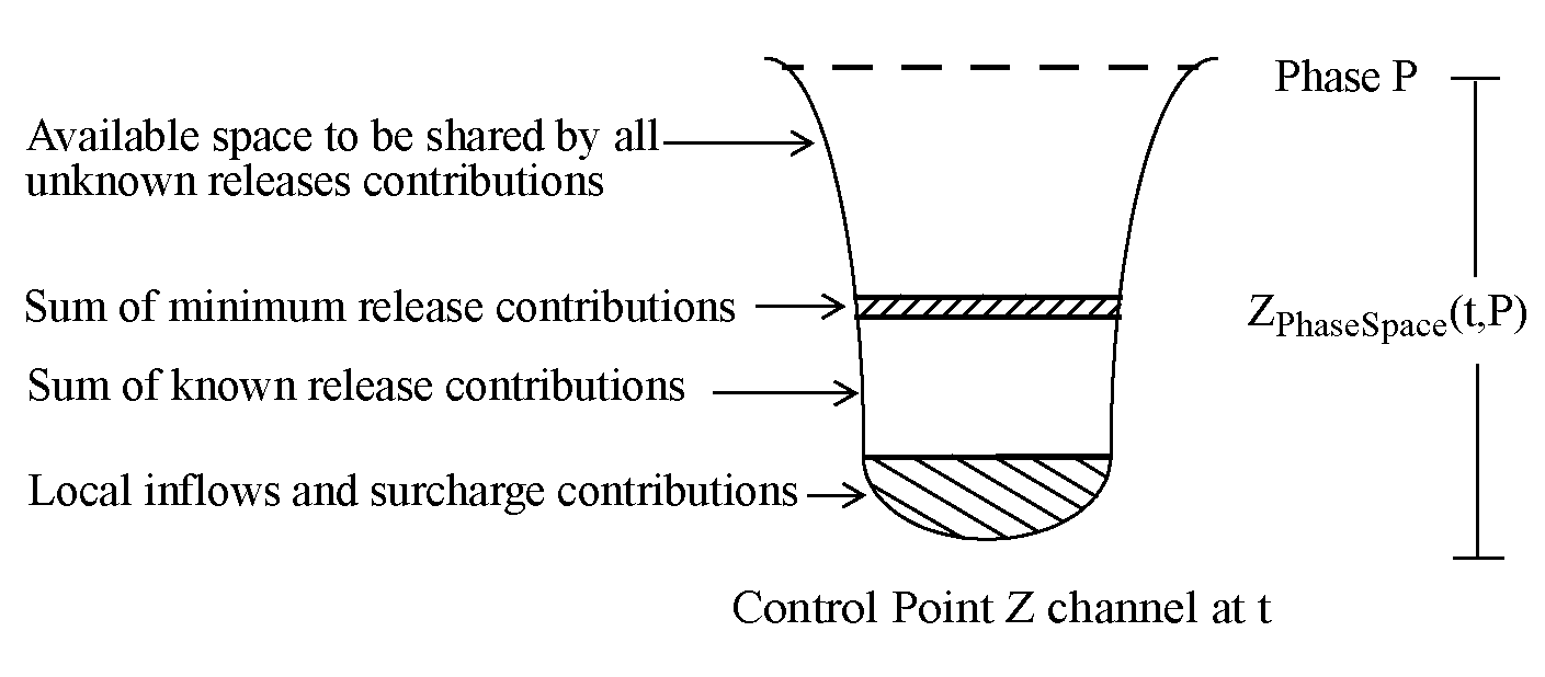
a. Calculate the reservoir’s phase space allocation at the current control point. The phase space allocation at each control point is calculated by determining which reservoir releases contribute to the water in the control point. The contributing reservoir releases are determined from the control point’s reservoir list and the linear routing coefficients. Available space in the control point is calculated by taking the phase space hydrograph and subtracting out local inflows, all contributions of known reservoir releases, and minimum release contributions from reservoirs whose release is unknown. Known reservoir releases are considered releases that occurred before t - lag time from the reservoir to the control point. These are releases that have already been constrained by the current control point. Unknown reservoir releases are all reservoir releases occurring at or after t - lag time from the reservoir to the control point. These are releases that have not yet been constrained by the current control point. The available space is then divided up to all unknown reservoir releases which will contribute the control point at the current timestep. The space is divided among reservoirs using the reservoirs’ linear routing coefficients and reservoirs’ lake character weight at the timestep t-1-lag time from the reservoir to the control point.
Figure 8.2
The lake character value is calculated by the reservoir as follows: The Lake Character is a weighting factor that will be determined for certain types of Reservoir Objects (Storage and Level Power Reservoirs) to be used as a means to balance all reservoirs in the same Operating Level. Once the Lake Character is known, it can be used in conjunction with other reservoirs of the same Operating Level to divvy up the available empty space at downstream control points. A reservoir’s Lake Character for each timestep is calculated by:

The coefficient is either the value in the Lake Character Coefficient scalar slot or the value in the Variable Lake Character Coefficient series slot if input for that timestep. RiverWare will check at each timestep if a value has been input in the Variable Lake Character slot. If valid, the Coefficient is the input value for some timestep from Variable Lake Character Coefficient. When NaN, the Coefficient is the value in the Lake Character Coefficient ScalarSlot.
The percentage of the flood pool that is currently occupied is calculated as follows:

This storage value takes into account the Surcharge Release determined for the current timestep. The Top of Flood Control Pool Level and Top of Conservation Pool Level are required input. The storage corresponding to these level will be determined from an interpolation of the Elevation-Volume TableSlot.
b. The proposed flood control release slot for each reservoir is then set to the minimum of the current value of the proposed flood control release or the phase space allocation at the control point divided by the linear coefficient. Dividing the allocation by the linear coefficient results in a release value that will wholly fill the allocated space. Recall the minimum release contribution was subtracted out of the available phase space, ensuring that space would be available for all minimum releases.
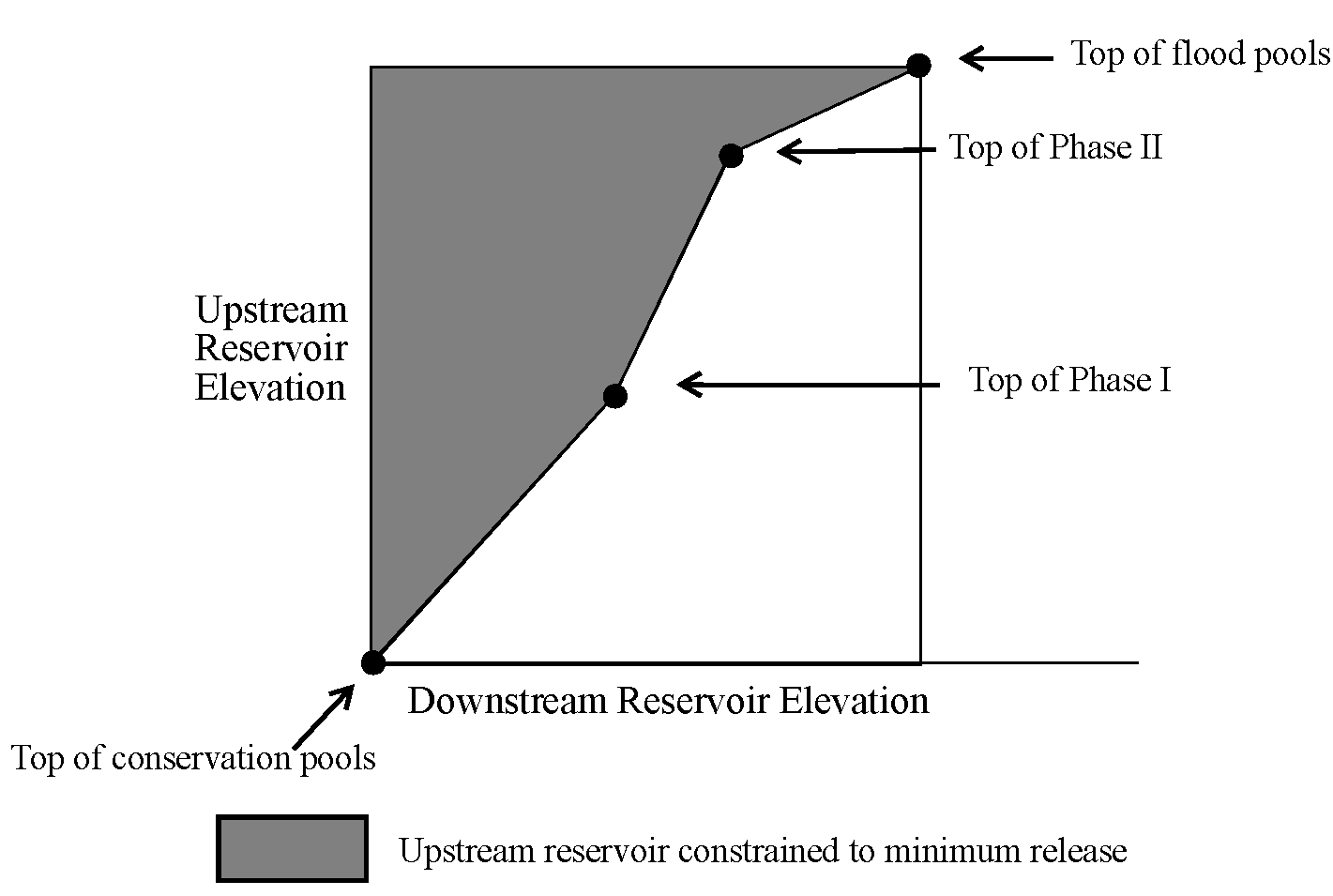
c. If the control point lists a reservoir directly upstream (that is, there is no time lag from the reservoir to the control point) and the reservoir has upstream tandem reservoirs, the control point may constrain upstream tandem reservoirs to their minimum release. Two reservoirs which are located so that a release from one becomes the inflow of the other are in tandem. The upstream reservoir releases will be set to the reservoir’s minimum release if the two reservoirs are out of tandem balance. A tandem balancing curve is constructed for each pair of tandem reservoirs by interpolating straight lines between the following points calculated from the tandem operating levels table slot and the tandem operating aberrations slot:
• Top of flood pool
• Top of Phase II
• Top of Phase I
• Top of conservation pool
If more water is stored in the downstream tandem reservoir than indicated by the tandem balance curve then the temporary release from the upstream reservoir will be set the minimum release. Given a reservoir D and its tandem upstream reservoir U. The tandem upstream reservoir is constrained to its minimum release if the point (DPoolElevation(t-1), UPoolElevation(t-1-lagTime)) lies within the shaded area. If the point lies in the unshaded area, the flood control release is the same as the parallel case.
Figure 8.3
d. If not all of the control point’s available phase space was taken by its reservoirs’ releases (one or more of the reservoirs may have been constrained upstream) the phase space allocation is repeated with all reservoirs which are not constrained upstream, considering all releases constrained upstream as known releases. This process is repeated until the entire phase space is allocated for the current timestep or until all of the current control point’s reservoirs are found to be constrained upstream.
Note: See the notes regarding the flood control methods in general, above.
This method uses a series of passes over successively lower operating levels (called balance levels in this context), in which it attempts to reduce all the reservoirs in the subbasin to the operating level of the pass. It attempts to release as much water as feasible as soon as possible.
A set of criteria is applied, reducing the potential release from each full reservoir, to meet all the following goals:
• Flooding does not occur downstream at the control points to which this reservoir routes1.
• Water is not released from the reservoir’s conservation pool, and the release schedule does not rely on any water being released from the conservation pool in its projections.
• Priority is given to reservoirs based on their operating levels (“fullness”).
• Reservoirs subject to a key control point are left as balanced2 as possible, given the above.
• Flood pools are drained as soon as possible and within the forecast period, given the above.
• Reservoirs have a release schedule that is as smooth as possible, given the above.
See Beginning-of-run Checks Specific to This Method for details on the operation of this method.
When this method is selected, dependent method categories Balance Level Determination, Pass Behavior, Key Control Point Max Release, Key Control Point Space Use, Operating Level Mapping, Tandem Balancing, Modify Inputs to Two-Reservoir Midpoint, Tandem Storage Management, Tandem Storage Considered, Priority Determination, Reservoir Set, Smoothing Releases, Last Pass Timesteps May Increase apply, and Control Point Variable Routing Coefficients. They are described below.
Note: The Operating Level Balancing method was developed under the aegis of the U.S. Army Corps of Engineers - Southwest Division, with the expressed purpose of approximating algorithms and results of portions of the Corps’ SUPER suite of programs. Some of the methods described below (among those dependent on Operating Level Balancing) exist solely for the testing and acceptance phase of this project. Some of these methods and the slots associated with them may not persist in RiverWare, and are so indicated below. Other methods exist for the purpose of experimentation, to enable interested persons to study the effects and interactions of various algorithmic details. The defaults were chosen to match the SUPER behavior. See Flood Control in USACE‑SWD Modeling Techniques for details on using this method for USACE-SWD.
Note: Undocumented temporary slots may appear (with “Temp” or “Temporary” in their names) in various releases of RiverWare, and may disappear later, for the reasons stated in the previous note. Such temporary slots are not stored with a model, and are not deemed available to users for use in rules, user-defined accounting methods, or for any other purpose. In RiverWare 6.1, many of the Temp slots were converted to regular slots but then made invisible. These invisible slots but can be viewed in the Special Results details on the Model Run Analysis tool; see Model Run Analysis—Special Results Details Dialog in USACE‑SWD Modeling Techniques.
Slots Specific to This Method
Forecast Period
Type: Scalar Slot
Units: NONE
Description: Timesteps in the period for which forecast data are available.
Information: Minimum value of 1. Can be propagated from the subbasin to its members. All subbasin members with this slot must have the same value in the slot.
I/O: Required input
Links: Not linkable
Balance Period
Type: Scalar Slot
Units: NONE
Description: Timestep in the future (origin 1—that is, 1—means the current simulation timestep) at which the forecast storage in the flood pool determines the amount of water to be released over the forecast period by the flood control algorithm.
Information: Minimum value of 1. Less than or equal to the value of the Forecast Period. Values must match on all objects in the subbasin that have this slot. Can be propagated from the subbasin to its members.
I/O: Required input
Links: Not linkable
Top of Conservation Pool
Type: Scalar Slot
Units: NONE
Description: Operating level associated with the top of the conservation pool of every reservoir in the subbasin (all reservoirs in the subbasin must have the same value for this slot).
Information: Also known as target operating pool level, since this is the preferred, or target, level for all reservoirs. This level is also the bottom of the flood pool. Can be propagated to every subbasin member that has this slot.
I/O: Required input
Links: Not linkable
Top of Flood Pool
Type: Scalar Slot
Units: NONE
Description: Operating level associated with the top of the flood pool of every reservoir in the subbasin (all reservoirs in the subbasin must have the same value for this slot).
Information: Must be greater than the Top of Conservation Pool. Used to compute surcharge releases. Can be propagated to every subbasin member that has this slot.
Highest Operating Level
Type: Scalar Slot
Units: NONE
Description: The highest operating level that is valid for every reservoir in the subbasin. The Operating Level Balancing method will not consider operating levels higher than this when it attempts to balance reservoirs.
Information: Used in the Two-Reservoir Midopoint method of the Tandem Balancing category (dependent on the Operating Level Balancing method selection). Every reservoir in the subbasin must have an Operating Level Table whose domain covers this operating level because the Two-Reservoir Midpoint method looks up storages associated with levels up to and including this.
I/O: Required input
Links: Not linkable
Lowest Operating Level
Type: Scalar Slot
Units: NONE
Description: The lowest operating level that is valid for every reservoir in the subbasin. The Operating Level Balancing method will not consider operating levels lower than this in its attempts to balance reservoirs.
Information: Used in the Two-Reservoir Midopoint method of the Tandem Balancing category (dependent on the Operating Level Balancing method selection). Every reservoir in the subbasin must have an Operating Level Table whose domain covers this operating level. The Two-Reservoir Midpoint method looks up storages associated with this balance level on each reservoir in the subbasin.
I/O: Required input
Links: Not linkable
Routed Flow Tolerance
Type: Scalar Slot
Units: FLOW
Description: Performance tuning knob. Flow, due to a routed flood control release, below which it is not worth the computational expense to continue processing.
Information: When, during the computation of a prospective additional flood control release, the resulting routed flow at a control point is below this value, the method considers it to be zero, at (and downstream of) this control point.
I/O: Required input. Default value 0.000001 cms.
Links: Not linkable
Incremental Release Tolerance
Type: Scalar Slot
Units: FLOW
Description: Performance tuning knob. Magnitude of additional release (for a pass of the flood control algorithm) below which it is not worth the computational cost to consider.
Information: When, during the computation of a prospective additional flood control release, the additional release becomes limited to a magnitude below this, the additional release is taken to be 0.0.
I/O: Required input; default value 0.000001 cms.
Links: Not linkable
Beginning-of-run Checks Specific to This Method
Prior to the start of a run, the subbasin is analyzed and verified, at which time the following checks are made.
1. On the subbasin:
– The following slot values must be positive: Forecast Period, Balance Period, Highest Operating Level.
– The following slot values must be non-negative: Routed Flow Tolerance, Lowest Operating Level.
– The Balance Period must be less than or equal to the Forecast Period.
– The Highest Operating Level must be greater than the Lowest Operating Level.
2. On member reservoirs:
– The following slot values must be positive: Allowable Rising Release Change, Allowable Falling Release Change, Maximum Release Variation.
– The following slot values must be non-negative: all elevations in the Operating Level Table.
– For each date in the Operating Level Table, the elevations must monotonically increase with the operating level, and the Operating Level Table must cover the range Lowest Operating Level through Highest Operating Level (from the subbasin slots).
– Each reservoir must have the Operating Level Balancing method selected for the Flood Control Release category.
– (This is not a check, but an action taken:) A slot, Operating Level Storage Table, is created at this time. It is a direct mapping between operating levels and volumes, created from the Elevation-Volume Table and the Operating Level Table. For performance purposes, this table is used by the flood control and related methods in lieu of two table interpolations for mapping storage volumes to operating levels and back. Also, see the Conditional Operating Level category in Conditional Operating Levels for details on when this slot could be recomputed.
3. On member control points:
– The following slot values must be positive: Excepted Releases, if the control point has a flooding exception.
– The following slot values must be non-negative: elements of Routing Coefficients.
– If the control point is key, its Key Control Point Balancing method must be Operating Level Balancing.
– The sum of the elements of the Routing Coefficients vector for each Upstream Reservoir must be within Routed Flow Tolerance of 1.0.
– The Empty Space slot must be valid, which means that a method other than None for Regulation Discharge must be selected. This slot determines how much water can flow at a control point without causing flooding. Flooding is defined as flow exceeding the regulation discharge.
– Each control point must have the Operating Level Balancing method selected for the Flood Control Release category.
4. Relationships among slot values of objects in the subbasin:
– The following slots, when instantiated on members, must match those of the subbasin: Balance Period, Forecast Period, Top of Conservation Pool, Top of Flood Pool.
5. Relationships among objects in the subbasin:
– Each reservoir has a member control point “immediately” (considering only reservoirs and control points) downstream, which is called its “output gage control point”. The Routing Coefficients vector from the reservoir to its output gage control point is exactly { 1.0 }.
– All subject reservoir of a key control point (those named in the control point’s Key Control Point Reservoirs slot) must be members of the subbasin and upstream of the control point.
– When the selected method for Key Control Point Space Use is Key Control Point Balancing Share, there cannot be non-subject reservoirs interposed between a key control point and any of its subject reservoirs. This is because the non-subject tandem may take on storage of water released from a subject reservoir upstream, but be unable to release it. When the selected method is First-Come First-Served, it doesn’t matter, as all reservoirs have equal access to the key control point’s empty space.
– Every reservoir in a control point’s Upstream Reservoirs slot must be a subbasin member and must be upstream of the control point.
Note: There is no beginning-of-run check that the Key Control Point Reservoirs are among the Upstream Reservoirs, but the Key Control Point Balancing method Operating Level Balancing will issue a fatal error if they are not.
Note: If a given control point has the Compute Aggregate Coefficients method selected in the Variable Routing Coefficients category, the temp Routing Coefficients slot will be used in place of the Routing Coefficients slot in all calculations. This slot is populated at the beginning of the timestep based on the flows in the system. See the Compute Aggregate Coefficients method documentation in the Control Point Variable Routing Coefficients category below.
Subbasin Example
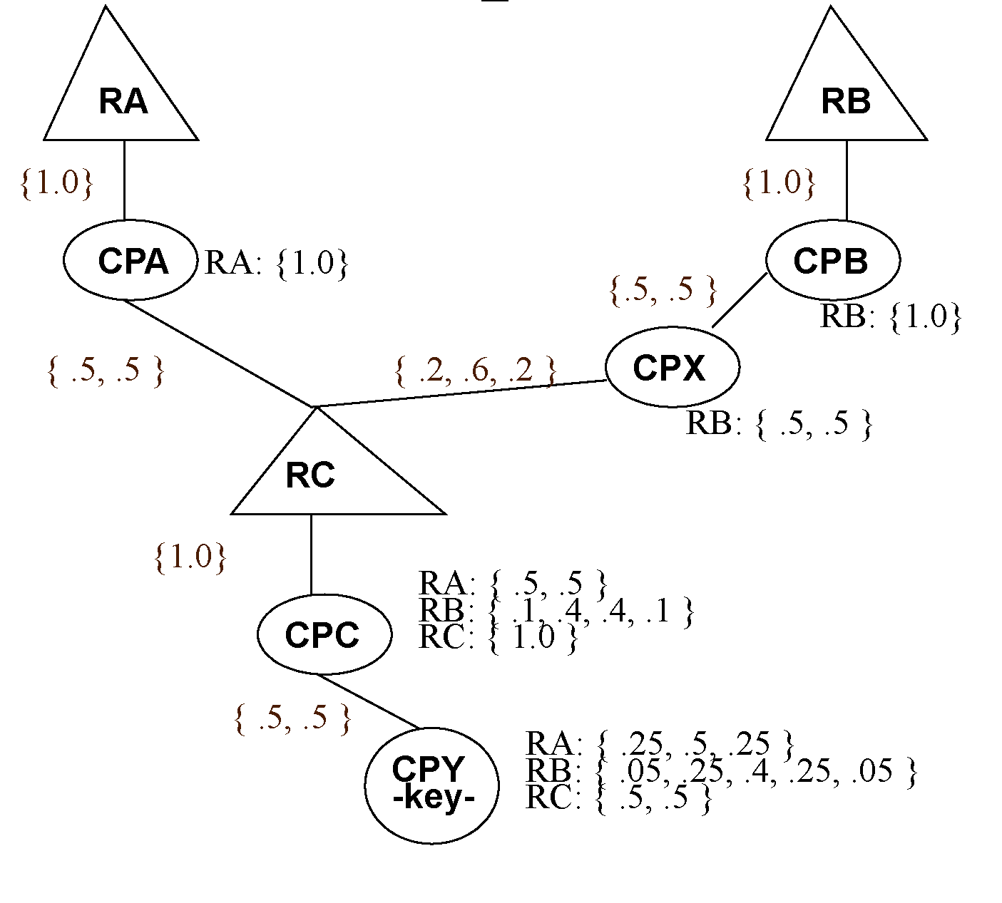
For illustrating the behavior of this method with examples, we refer to the following simplified subbasin (with only reservoirs and control points extracted; Reaches and other objects are not of interest to the flood control algorithm and so are not considered in any discussion of the flood control algorithm). This example subbasin, illustrated below, contains three reservoirs, RA, RB and RC. Each reservoir has an “output gage control point”, CPA, CPB, CPC, respectively. Two more control points, CPX and CPY are in the subbasin. In the subbasin from which this is extracted, there would be Reaches between CPB and CPX, and between CPC and CPY. There would also be a confluence above RC, possibly with Reaches between it and CPA and between it and CPX. During simulation, the dispatching of reaches would affect the routing. which is incremental (one reach at a time), but during execution of the flood control rule, the linear routing coefficients on the control points are used to approximate the composite (cumulative) routing between reservoirs and control points.
For the purpose of illustration, we assume that this subbasin has the following attributes:
• 1 Day timestep,
• Forecast period of 5days,
• Balance period of 3 days,
• Top of the conservation pool at operating level 5.0,
• Hypothetical units, in which 1 unit of volume == 1 unit of flow (for simplicity)
• Hidden reaches with routing coefficients, as shown in Figure 8.4
Figure 8.4
Method Details
The Operating Level Balancing method first determines if flood control is needed. If no reservoirs in the subbasin are forecast to be in the flood pool on the current simulation timestep, it returns with no flood control releases for any of the reservoirs in the subbasin.
Note: If a reservoir in the computational basin is disabled and is set to Pass Inflows (see Pass Inflows), the reservoir is not considered in the computations below. The reservoir will pass the flows through including any upstream releases that could possibly have been held as tandem storage.
If flood control is needed, the method initializes the flood control release schedule3 for each reservoir to zero: no flood control release on any timestep of the forecast period. It then invokes the selected Key Control Point Balancing method on each of the key control points in the subbasin. After this, the method selects a set of balance levels to use to drive the algorithm. This set is determined by the selected method in the Balance Level Determination category (q.v., below). The set is sorted in descending order (duplicate values are removed) and preserved so it can be returned to the calling rule/function to set on the Target Balance Level slot.
The flood control method then runs one or more “passes” over the reservoirs in the subbasin. There is one pass for each balance level in the above-mentioned set, and an additional “final” pass associated with the operating level that is the Top of Conservation Pool. The goal of each pass is to determine the maximum release that each reservoir can make on each timestep of the forecast period, to bring its forecast operating level to the balance level of the pass as soon as possible4. No attempt is made to reduce a reservoir below the level of the pass.
At the beginning of each pass, the method determines the set of “full” reservoirs, namely those whose forecast operating levels (at the end of the balance period) exceed the balance level of the pass 5. The set of full reservoirs is sorted by fullness (fullest one first).
The full reservoirs are considered in order, and for each full reservoir there are two steps to compute a release schedule. Remember that all the actions described here are on intermediate (temporary or invisible) slots; the simulation state of objects is not changed by the flood control method. (Empty space and storage slots are not changed.)
1. Undo the proposed releases from the prior pass (if any), freeing space at control points and removing tandem storage at tandem reservoirs. This step is not necessary if accumulating additional releases on each pass (Pass Behavior method selected is Compute Additional Release).
2. Loop over the timesteps in the forecast period, computing a tentative release for each timestep. In this loop are two steps:
• Compute a tentative release for the full reservoir for the forecast timestep in question, based on empty space at the downstream control points, on our ability to store water in a downstream tandem reservoir, and on constraints of the full reservoir; and
• “Apply” that tentative release, updating the empty space at downstream control points and storages at downstream reservoirs.
RA is forecast to be at level 10.2, RB at 8.9, RC at 9.5. The key control point, CPY, assigned balance level 9.0 to reservoirs RA, RB and RC, and so its balance level for the current timestep is 9.0. The balance level set is { 9.0, 5.0 }. There are three passes, one at 9.0, one at 5.0 and a “final” pass at 5.0, in which certain constraints, described below, are removed. On the first pass, the algorithm proposes release schedules for RA and RC that will bring them down as close to operating level 9 as possible in 5 days, given empty space constraints at control points. It considers RA before RC because RA is forecast to be “fuller” (at a higher operating level). On the second pass, the algorithm proposes releases for RA, RC, and RB, to bring them down to operating level 5.0 while still respecting all the constraints of the first pass. On the final pass, all reservoirs are considered, with the goal of bringing them to level 5.0, with slightly different constraints, as described below.
Downstream Objects that Constrain a Full Reservoir’s Release
The objects that constrain a reservoir’s release are those reachable by water routed within the forecast period. For the purpose of the flood control method, water travels only as far as
• there are control points with routing coefficients from that full reservoir, and
• it can travel within the forecast period, and
• it will result in at least Routed Release Tolerance cms on the timestep in question.
Note: This is internal units.
If there were no routing coefficients at CPC for routing from RA to CPC, the flood control algorithm would stop checking constraints at CPA, even if control points downstream of CPC had routing coefficients for releases from RA. If the routing coefficients for RA to CPC were { 0,0,0,.5,.5 }, no releases after the 2nd day would be considered from CPC on downstream, because no water from such releases would reach CPC or beyond within the forecast period. Finally, if the Routed Release Tolerance were 0.000001 cms, and a release were to route to a control point but the arriving flow were to be less than 0.000001 cms, the flood control algorithm would stop at said control point. Thus, the Routed Release Tolerance can be used to tune the algorithm - to make it run faster, but with less precision.
The flood control algorithm does not check for consistency of the linear routing coefficients with the simulation routing. If the linear routing coefficients used by the flood control do not approximate the routing used in simulation, results may be of low quality. Similarly, if the routing coefficients at two control points are inconsistent, RiverWare will not notice.
Routing coefficients from RA to CPC could be {.5,.5} and from RA to CPY could be {.8,.2}, and RiverWare would not notice. It is entirely up to the modeler to see that the coefficients are consistent with each other and with the simulation routing methods.
The routing coefficients on the Reach between CPA and RC might be {.1,.2,.3,.4}, and all else as described in the reference subbasin. RiverWare would use the routing coefficients on the reach during simulation, and the routing coefficients on the control points for flood control. The fact that they don’t match would not be discovered by RiverWare. The Reaches might not use linear routing at all. RiverWare would have no way to tell if the linear routing used in flood control is an “acceptable” approximation of the (possibly non-linear) routing selected on the Reaches and used during simulation.
Empty Space Restrictions at Control Points
Limited channel (empty) space at downstream control points may reduce the proposed release. The available empty space on a pass is determined as follows.
• On all passes, all empty space at non-key control points is available on a first-come, first-served basis.
• Space at key control points is reserved for use by subject full reservoirs on passes prior to the final pass. This allocation of space is respected on these passes, unless overridden by the selected method in the Key Control Point Space Use category (q.v., below). See below for a discussion of the allocation of water stored in downstream tandem reservoirs.
• On the final pass, all empty space at all control points that has not been used heretofore is available on a first-come, first-served basis.
The key control point balancing method on CPY apportioned its empty space as follows: 60% to RA and 40% to RB. With three passes, at operating levels 9.0, 5.0 and 5.0, on the first two passes (9.0 and 5.0), RA releases can consume at most 60% of the empty space at CPY on any day of the forecast period, while RB can consume at most 40%. On the final pass, any unused space at CPY is available to both RA and RB. Empty space at CPC is available to RA and RB on all passes because CPC is not key.
“Trim” (Max Release Variation) and Empty Space
When considering empty space at a control point, the method computes an upper bound on the flood control release for each timestep in the forecast period. The upper bound is the maximum amount that can be used as the first ordinate in a stepped-down release hydrograph from the timestep under consideration through the end of the forecast period, with the full reservoir’s Maximum Release Variation (so-called “Trim” value) defining the magnitude of the reduction in this hydrograph between timesteps, and when this hydrograph is routed to the control point, all the resulting flow for the rest of the forecast period will fit in the empty space available at the control point. This stepped-down hydrograph is computed without regard to the goal release volume; it merely results in an upper bound on the release at each timestep. (This is a heuristic method of smoothing the release schedules. There is no guarantee that the second and succeeding timesteps of the stepped-down hydrograph will approximate the release hydrograph ultimately resulting from the flood control operations.)
We are proposing a release from RB. For the purpose of this example, let us assume that below CPX, no other constraints reduce a release, that is, this example considers only the effects of CPB and CPX. RB has volume of 150 units to release to bring it down to the goal balance level for the pass. RB has a Max Release Variation of 10 flow units per timestep. Empty space at CPB for the forecast period is { 50, 50, 50, 50, 50 }. For the first forecast day, the empty space at RB would permit a stepped-down release hydrograph of {50, 40, 30, 20, 10}, so it proposes a release of 50 units. For the second day, the remaining empty space at CPB would then be { 0, 50, 50, 50, 50 }, so it proposes a release of 50 units again. Now the proposed release schedule is { 50,50, 0, 0, 0 } and the proposed empty space at CPB is {0,0,50,50,50}. Thus, CPB will impose the same upper bound on each day’s release from RB.
Continuing the above example, we now consider the empty space at CPX, which is { 50, 60, 40, 50, 50 }. For the first day, the stepped-down hydrograph would be 55, 45, 35, 25, 15}, which, routed, yields {27.5,50,40,30,20}, limited by day 3. Since the release is already constrained to 50 units on each day, CPX does not impose any constraints on the RB release schedule for the first day. Assuming the release from RB for the first day is indeed 50 units (after considering all control points and all other constraints), arriving at CPX as {25,25,0,0,0), on the second day the resulting free space at CPX would be {25, 35, 40, 50, 50}. This empty space dictates a stepped-down hydrograph for day 2 of { 0, 45,35,25,15}, resulting in an arrival hydrograph of { 0, 22.5, 40, 30, 20 }, restricted by day 3. Thus, the upper bound of 45 is imposed on the release for day 2. Assuming that holds, we route it to CPX, and it arrives as {0,22.5,22.5,0,0}. This leaves empty space for day 3 at { 25,12.5,17.5,50,50}. This empty space dictates a stepped-down hydrograph for day 3 of {0,0,35,25,15}, which, routed to CPX gives an arrival hydrograph of {0,0,17.5,30,20}, being restricted by day 3. Thus, the upper bound of 35 is imposed on day 3, which we assume remains the release for day 3. Routed to CPX, it arrives as {0,0,17.5,17.5,0), which reduces the empty space to {25,12.5,0,32.5,50}. The day 4 hydrograph is then { 0,0,0,55,45}, routed to CPX arriving as 0,0,0,27.5,50}, being restricted by day 5. Thus, the day 4 upper bound is 55, and if it ends up being released, it routes to CPX as {0,0,0,,27.5,27.5}, leaving empty space of {25,12.5,0,5,22.5}. This empty space dictates a day 5 hydrograph of {0,0,0,0,45}, which gives the upper bound of 45 for day 5. Thus control point CPX imposes limits of {55, 45,35,55,45}, and the release schedule is {50,45,35,55,45}.
While the above consideration of empty space guarantees that no release will cause flooding downstream, given the routing information and the forecast period limitations at hand, the following circumstances could cause flooding downstream at simulation time:
• the routing coefficients used by the flood control algorithm do not closely approximate the routing used during simulation, or
• the forecast period is considerably shorter than the effect of the routed releases at simulation time, or
• the model does not contain routing coefficients for control points reached within the forecast period by releases from reservoirs above, or
• there is a Flooding Exception relationship between a control point and a reservoir (see the Flooding Exception category on a control point for details).
Constraints of the Full Reservoir
The proposed release at any timestep in the forecast period will not exceed the release at the prior timestep plus the full reservoir’s Allowable Rising Release Change. When computing this constraint on the release, surcharge and flood control minimum releases are considered.
RA’s Allowable Rising Release Change (ARRC) is 20. Computing RA’s optimal release for the first day yields a release of 100. The total release (surcharge release plus flood control release) made on the prior simulation timestep was 75, so RA will not release more than 95 today (surcharge and flood control releases combined). After applying all other constraints, we end up with a release for today of 55. That means that the second forecast day’s release will not exceed 75, and so on throughout the forecast period.
The algorithm tries to assure, but does not guarantee, that the proposed releases in the forecast period do not drop by more than the full reservoir’s Allowable Falling Release Change. This constraint is applied by computing a stepped-down hydrograph that releases the goal volume for the timestep (based on the difference in storage between the forecast operating level at the end of the balance period and the balance level of the pass) over the remaining timesteps in the forecast period, with a reduction at each timestep of exactly the Allowable Falling Release Change within the forecast period (the last ordinate may exceed the Allowable Falling Release Change). The first ordinate in such a hydrograph is used as an upper bound on the release for the timestep under consideration. Of course, a release at some timestep may be forced to zero by sudden inflows at a downstream control point, and this can cause the Allowable Falling Release Change constraint to be untenable for that timestep. The upper bound computed on the first timestep (which uses the goal volume that is the entire flood pool’s contents above the balance level of the pass) is applied to every timestep of the forecast period. Thus, the first timestep of the forecast period has one such upper bound applied, while the rest of the timesteps have two such upper bounds applied (one for the whole volume to release, and one for the remaining volume to release at that timestep).
RA’s Allowable Falling Release Change (AFRC) value is 10 flow units per timestep. RA is forecast to have150 units of flood pool volume at the end of the balance period, so 150 units is the release goal on a pass at balance level 5.0. The stepped-down hydrograph computed for 150 units volume for the first timestep is {50, 40, 30, 20, 10}, which releases all the volume in the forecast period. Thus, 50 is an upper bound on the first day’s release. Having ultimately released 40 on the first day, due to space restrictions downstream, we compute a new hydrograph for the second day, to release 110 units in the 4 remaining days. This hydrograph is {42.5, 32.5, 22.5, 12.5}.
Note: The last day’s ordinate may exceed AFRC, because our goal is first to release all the water within the forecast period, knowing that forecasts far out in the forecast period are dubious in any case.
The second hydrograph imposes an upper bound of 42.5, in addition to the upper bound of 50 on the release for the second day. Assuming we could ultimately release 41 units on day 2, we have for the third day 110-41=69 units to release. We compute a hydrograph for the third day: {33, 23, 13}. Thus the third day’s release is subjected to the upper bound of 50 and the upper bound of 33. If a downstream control point imposes a limit of 0 on the third and fourth day releases, we will still have 69 units to release on day 5. This will give us a stepped-down hydrograph of {69}, and the upper bounds of 69 and 50 will apply to day 5. Thus, the upper bounds for each of the days for this constraint will be: {50,42.5,33,39.5,50}.
The proposed release at the simulation timestep cannot exceed the spillway capacity, as determined by the reservoir’s utility method getMaxOutGivenIn(). (This constraint is not applied to forecast timesteps after the first, that is, after the current simulation timestep.) If part of an upstream reservoir’s proposed release is to flow through a downstream tandem reservoir (results in a so-called “through release”), the downstream tandem’s spillway constraint is applied to the amount of the through release arriving on the simulation day plus other inflows so-far computed, along with other releases so-far computed for the tandem. Thus, the spillway constraint on the tandem may restrict flood control releases from upstream reservoirs.
RA can release 100 units, and RC cannot store any water (having stored plenty from RB). Routing 100 units from RA to RC, we get {50,50}, and we then apply the spillway constraint at RC, considering the 50 arriving as being in addition to any other inflows at RC, and considering any other proposed releases from RC. If the release from RA, upon flowing through RC, could exceed the spillway capacity of RC, RA’s release will be reduced accordingly.
The proposed release at a timestep cannot dip into the full reservoir’s conservation pool on that forecast timestep. This constraint can be applied to every timestep in the forecast period, or only to the first timestep, based on the method selection in the Tandem Storage Management category (q.v.).
If the Key Control Point Max Release category selection is Max Release Applies, the maximum flood control release constraint applies: on all passes but the last, a reservoir’s proposed release cannot exceed the reservoir’s Max Flood Control Release on any timestep. This value is computed by the Key Control Point Balancing method. If a reservoir is not subject to a key control point, this constraint has no effect.
Key control point CPY assigns to RA a maximum release of 40 units, and to RB a maximum release of 30 units. If we have three passes, at levels 9.0, 5.0 and 5.0, on the first two passes, RA will release no more than 40 units on any day of the forecast period. RB will not release more than 30 units on any day of the forecast period. Thus even though RA may be forecast to be significantly higher than RB, it may not be able use all the downstream channel space otherwise available to it. Only on the final pass will these limits be lifted, and RA will be free to consume all remaining channel space, subject to its other constraints. Assuming that the key control point allocates these maxima in proportion to the fullness of the reservoirs, using the maxima may have the effect of allowing each reservoir to release something each timestep, rather than allocating all channel space to RA today, leaving RB “fuller” tomorrow, allocating all channel space to RB tomorrow, leaving RA “fuller” the next day, and so on (causing undesirable oscillating behavior). Of course, the effect depends on the key control point balancing method selected.
On the last pass, the release schedule at timesteps after the first are subjected to another upper bound, which is the larger of
• the value proposed on the prior pass for the timestep, and
• the value proposed on this pass for the prior timestep minus the trim value (Maximum Release Variation slot).
This constraint can be overridden by selecting the Entire Forecast Period method of the Last Pass Timesteps May Increase category.
RB is forecast to be at level 10.0 and RC is forecast to be at level 5.0 at the end of the balance period. The key control point balancing method assigns level 7.0 to all three reservoirs. On the first pass, at balance level 7.0, RC takes on 100 units from RB, released as { 40, 30, 20, 10}. Since the forecast period is 5 days long, the arrival hydrograph for this release schedule from RB is {4, 19, 30, 25, 15}, but because we consider only that water that arrives within the balance period, we account for only the 53 units arriving on days 1-3, leaving 47 units that arrive after the end of the balance period. Thus, in future calculations based on the forecast storage in RC, 53 units of volume will be added to RC’s forecast storage. RC will be free to release on day 1 an additional 4 units of volume, and on day 2 an additional 19 units of volume, and so on through the forecast period. If the Two-Reservoir Midpoint method is selected, the starting volume for RC will henceforth include 53 units of volume above its forecast volume at the end of the balance period.
Storing Water in Downstream Tandem Reservoirs
All or part of a proposed release may be stored in downstream tandem reservoirs if the downstream reservoir is not Surcharging (Surcharge Release equals zero or is not valid) at the current controller timestep. Such tandem storage is determined as follows.
• A downstream reservoir will store water to increase its forecast operating level to the smaller of the pass’s balance level and the tandem reservoir’s Target Balance Level (assigned by a controlling key control point). If a reservoir is not subject to any key control point and thus not given a balance level, the Top of Conservation Pool value will be used for the assigned balance level and an error will be issued. This error terminates the run.
• A downstream reservoir may store additional water if the Two-Reservoir Midpoint method is selected in the Tandem Balancing category; see Tandem Balancing.
There are four passes at balance levels 9.0, 8.7, 5.0 and 5.0. RC, subject to more than one key control point (not shown in the example subbasin), has been assigned a balance level of 8.7. On the first pass (9.0), RA may store water in RC to bring RC up to the larger of 9.0 (balance level of the pass) and 8.7 (balance level assigned RC). On the second pass, RC will accept water to bring it no higher than 8.7 again. On the last two passes, it will accept no water, unless it is forecast to be in the conservation pool at the end of the balance period, in which case, it will accept water to fill the conservation pool. If the Two-Reservoir Midpoint method is selected, RC will, in addition, agree to accept more water. Let us assume, as in a prior example, that RA is forecast to be at 10.2, RB at 8.9, and RC at 9.5. RC will accept, from RA, that volume of water that, if instantaneously moved from RA to RC, would put RC and RA a the same operating level. That level will be somewhere between 10.2 and 9.5. RC will not initially accept any water from RB because RB is forecast to be lower than RC. If, on the first pass, RC is able to release enough water to bring it below the ending operating level of RA at the conclusion of the pass, RC will accept water from RB.
When the Key Control Point Space Use method is Key Control Point Balancing Share, and water is moved from a full reservoir to a tandem, ownership of key control point shares of the empty space are transferred from the full reservoir to the tandem in amounts equal to the resulting inflow at the tandem for each timestep of the forecast period. This allows the tandem to release the water through the key control point later, all else permitting. Transfer of such ownership applies only to water to be stored in the flood pool (not to water to be stored in the conservation pool, as it will not be drained by the flood control algorithm). This transfer of ownership is not necessary and is not computed when the Pass Behavior selection is Undo and Recompute Max Release.
This example applies only when Pass Behavior is Compute Compute Additional Release. On the first pass, RA releases 100 units of volume to be stored in RC, as follows: {50,30,20,0,0}. The key control point, CPY, has allocated to RA {30, 30, 30, 30, 30}, to RB {10, 10, 10, 10, 10} and to RC {20, 20, 20,2 0,20}. Having stored 100 units of RA’s water in RC, on a later pass we might be able to release some or all of that 100 units from RC, but because that water originated at RA, we transfer its ownership to RC. Routing the release hydrograph to CPY, we get {12,5, 32.5, 32.5, 17.5, 5}, so we transfer such units of water in CPY’s accounts. Now CPY has allocated to RA: {17.5, 0, 0, 12.5, 25}, and to RC: {32.5, 50, 50, 37.5, 25}.
The quantity of water scheduled for tandem storage and accounted for in the tandem reservoirs depends on the method selection in the Tandem Storage Management category. For details of the accounting, see the method descriptions, below.
Note: See the notes regarding the flood control methods in general, above.
1 Except when permitted at a control point by means of a flooding exception (method selection) at that control point.
2 With a minimal spread in operating levels
3 By “schedule”, we mean a proposed release for each timestep in the forecast period. Only the first timestep’s release will be simulated after the flood control rule function returns, but the flood control algorithm proposes a schedule for the entire forecast period to attain smoothness in release hydrographs and to respect priorities in the presence of routing.
4 The method determines a reservoir’s excess water, VOL, which is the volume of water in the reservoir at the end of the balance period that is above the balance level of the pass. The goal is to release VOL over the forecast period, but as soon as possible. There is no guarantee that the entire VOL will be released by the end of the balance period.
5 As the reader will see, user-selectable methods, described below, modify the meaning of a “forecast operating level at the end of the balance period”. For the purpose of this discussion, think of it as the forecast storage at the end of the balance period as computed before the flood control method was called, plus any water proposed for release from an upstream reservoir on a prior pass and arriving for storage within the balance period, minus water proposed for release within the balance period on any prior pass. Methods that modify its meaning include Operating Level Mapping, Tandem Balancing, Modify Inputs to Two-Reservoir Midpoint, Tandem Storage Management, Tandem Storage Considered.
Revised: 06/04/2022