
Mixed-integer Programming
Some user-selectable engineering methods require a mixed integer programming solution. The Unit Power Table method, for example, requires integer programming to model the start-up and shut-down of individual turbines. Mixed integer programming adds substantial computational time to an Optimization model.
Note: It is recommended that users contact RiverWare Support before attempting to use methods that require mixed-integer programming. Inquiries can be sent to: riverware-support@colorado.edu
Mixed Integer Programs are optimization problems that contain both continuous and integer variables. In the river and reservoir modeling context, many of the variables are continuous. For example, outflow, pool elevation, and storage are all continuous variables. In contrast, hydropower turbines are operated such that a unit is either off or fully on. Thus, the Unit Power Table method has introduced some integer and binary (zero or one) variables. More specifically, the number of units generating at a given plant during a given time step is an integer variable and the decision to operate a single unit is a binary variable; the unit is either off or on. The modeling of integer and binary variables is sufficiently similar that the term integer is used to refer to both integer and binary variables.
Integer variables are also used to model discontinuities. For example, avoidance and cavitation zones are regions where power cannot be generated without damaging the equipment. These zones create a discontinuity in the power curve, and integer variables are used to model this discontinuity.
RiverWare solves this using Mixed Integer Linear Programs, but we will generally omit the word linear. The linear restriction reflects the fact that all non-linear functions have been replaced by linear or piecewise linear functions. The use of linear approximation allows the optimization to solve faster. We will also omit the word mixed and refer to Mixed-integer Linear Programming as simply Integer Programming.
Integer Programs are more difficult to solve than linear programs. For this reason, RiverWare has limited use of integer variables and the heuristic solution methods used are discussed in more detail in the rest of this section.
Variables That Bring Integer Programming Into the Problem
Two conditions are necessary for Integer Programming in RiverWare; integer programming is only allowed in the lowest priority policy and the policy must directly or indirectly use integer variables.
Integer Programming is limited to the lowest priority for performance reasons. To include integer variables at additional priorities would lead to what it called Integer Goal Programming (IGP). While there is no theoretical barrier, IGP is too computational challenging at this time. Consequently, RiverWare only allows integer variables in the final priority. If integer variables are referenced within a previous objective, RiverWare will relax the integrality constraints and solve the relaxed linear programming problem.
If a RiverWare policy doesn’t reference integer variables then integer programming is not used. Currently the only source of integer variables is the Unit Power Table and related methods (see Unit Power Table). Therefore, if only plant power methods are selected, integer variables will not be introduced and RiverWare will be solved as a Linear Goal Program.
The integer variables can be introduced either by directly referencing them in policy or by indirectly referencing them in policy. Integer variables are typically introduced indirectly by a user policy that optimizes the economic value of power using slots on the model’s Thermal object. During optimization, these slot variables will be replaced with equivalent expressions involving Power and related quantities on the individual power reservoirs. In this way, if the Unit Power Table method is selected, constraints which model unit level power concerns will be introduced into the optimization problem.
In addition, the user might write policy constraints which refer to binary quantities. For example, the user might want to forbid scheduling holes; that is, turning a unit off for a single time period. One normally thinks of writing this constraint as
Unit Is Generating [u,t] >= Unit Is Generating [u,t-1] + Unit Is Generating [u,t+1] ‑ 1
However, to avoid referencing future time periods they will need to write this as:
Unit Is Generating [u,t-1] >= Unit Is Generating [u,t-2] + Unit Is Generating [u,t] - 1
How Integer Programs Are Solved
Understanding the method used to solve integer programs is useful for understanding the solution information and adjusting parameters that control the solution process.
Integer programs are solved by first starting with a linear programming relaxation, for which integrality restrictions (i.e. that variables are either 0 or 1) are temporarily removed. From this relaxed solution two subproblems are created by branching on an integer variable. For example, the solver might branch on Unit 1 being used in the first period, with one branch requiring it to be used and the other branch requiring it not be used. This branching process can be continued with additional variables. The resulting process creates a tree structure that contains an optimal solution at one of the leaf nodes. Explicitly exploring the whole tree is impossible for all but the smallest problems. Fortunately, large portions of the tree can frequently be pruned off without exploration. The pruning is possible because the linear programming relaxation of a node in the tree may either be an integer solution, infeasible, or sufficiently suboptimal.
Timestep Approach
The integer programs formulated in RiverWare are sufficiently hard that an optional, but highly recommended heuristic has been added to speed up the solution process. The heuristic is an iterative timestep approach that focuses on solving early timesteps with integer variables while temporarily relaxing the integrality conditions for later timesteps. By relaxing the integrality constraints for most of the timesteps, the problem can be solved much more quickly. After obtaining a solution, the integer variables for the earliest timesteps are frozen at their integer values, and some previously relaxed variables are treated as integer variables. The problem is resolved, and the process continues until all timesteps have been modeled as integer variables and frozen. For each iteration the integer variables are constrained both by the frozen integer variables for previous time steps and the linear programming relaxation for future timesteps.
There are two time windows that are advanced at each iteration in this process, the range of (non-frozen) integer variables in the problem, and the possibly smaller range of integer variables that should be frozen after the problem is solved. The size of each of these windows is an important parameter of this process. By default, one time step is used for each of these time windows, but the user can increase these values by setting appropriate parameters, Mip Integer Window Size and Mip Freeze Window Size. If both variables are set to the number of timesteps in the run, then the MIP will be solved as a single problem containing all of the integer variables. At this time, we do not recommend increasing the window sizes beyond 1 because of the dramatic increase in computation time.
This process may find the optimal solution, but it is not guaranteed. During testing, the timestep approach has found high quality, feasible solutions in a fraction of the time to find an optimal solution and prove it is optimal.
Defining Constraints
See Mathematical Formulation of MIP for Unit Power for details on the mathematical formulation of the mixed integer programming to model unit power.
Additional Parameters for Controlling This Solution
CPLEX provides a variety of parameters to tune the solution of optimization problems. RiverWare makes these parameters accessible to the user. In addition, RiverWare has added some additional parameters to the list that are related to RiverWare’s use of goal programming and time windows. All of the parameters have default values determined by CPLEX or by CADSWES. In some cases CADSWES has replaced the default values of CPLEX parameters with values that have performed better for RiverWare models. These changes in the CPLEX parameters are in the cplex.par file packaged with RiverWare. Similarly, any non-default values for CADSWES parameters are contained in the goal.par file.
The vast majority of the parameters need never be examined, but some of them are potentially useful for integer programming. While branch and bound will theoretically find an optimal solution given enough time, the exponential growth of the search tree means that the time to do so is prohibitive for many practical problems. Instead, the tree can be used in a heuristic manner to find near optimal solutions. By limiting the number of solutions, the time allowed, and/or the optimality tolerance, the search can be terminated early with a good solution.
Setting Parameters
The parameters (both for CPLEX and RiverWare specific parameters) are set through the RiverWare interface. From the Run Control dialog, select Optimization as the controller and then select the menu option View > Optimization Run Parameters. From the Optimization Run Parameters dialog, select Set CPLEX and Goal Parameters. The parameters are organized by categories. Select the desired parameter and change the current value to the desired value. Select either Apply (to save and continue with other parameter changes) or Ok (to save and exit the parameter dialog). If you check the Save non-default settings to parameter file box these settings will be saved to a file called cplex.init.par, and this file will be used to initialize parameter settings for future RiverWare sessions.
Lower Cutoff Parameter
This parameter usually will not be effective when the timestep approach is used (see Timestep Approach). However, when optimizing the entire problem, this parameter can be very influential because of the structure of the branch and bound solution method. For maximization problems, the lower cutoff parameter will help prune the search tree until an integer feasible solution is found (an upper cutoff parameter can be used for minimization problems). Ideally, this parameter will be set high enough to eliminate large portions of the tree without eliminating all of the feasible integer solutions. Since the optimal integer solution isn’t known in advance, use of this parameter requires a little experimentation.
A starting point for the experimentation is the linear programming relaxation. By definition, integer solutions cannot improve on this value. For a maximization problem this means the optimal integer solution will be less than or equal to the linear programming relaxation and the lower cutoff parameter should certainly be set less than the objective function value for the linear programming relaxation. Our limited experimentation with test models suggests cutoff values ranging from about 90% of the linear programming relaxation to just below the linear programming relaxation.
Some experimentation is unavoidable with this parameter. If the lower cutoff value is set too high the search will end without a feasible solution. If the value is set too low (or there are too many time steps) the run will continue until some parameter stops the run or the user terminates the run. In both cases there won’t be an integer solution. If the problem is small enough to be solved, a reasonable cutoff value can typically be determined with a couple of tries.
The objective function of the linear programming relaxation can be obtained approximately by terminating the run with a little delay after the last objective has started. The delay is necessary to give CPLEX time to solve the relaxation. After terminating, the objective function of the best node in the tree will be printed in the RiverWare diagnostics window. This may be slightly less than the linear programming relaxation. In general this value will decrease as branch and bound proceeds. The number of nodes processed in the tree are also printed in the diagnostic. Unfortunately, for technical reasons the value can’t be printed while CPLEX is still running. The objective function is printed in optimization units, which are typically scaled from user units for numerical stability. For this reason, direct interpretation of the value is not advised. However, these are the same units that should be used for the lower cutoff value.
The lower cutoff parameter is in the MIP Tolerance Parameters category.
Limiting the Number of Solutions
Sometimes, branch and bound will find a good or even optimal solution early in an optimization and spend the bulk of its time proving optimality or making relatively minor improvements in the solution. Limiting the number of solutions can improve the solution time. However, testing has shown that setting this parameter overly low while using the timestep approach can lead to integer infeasibility in the middle of the timestep iterations.
The solutions parameter is in the MIP Limit Parameters category.
Time Limit
Optimization problems can take a long time to solve. A time limit parameter allows a solver to exit gracefully when the solver takes too long. For integer programs, exiting when the time limit expires will not generate an error if a feasible solution has been found. Thus, a time limit parameter can be used to truncate exploration of the branch and bound tree.
The time limit parameter in the General Parameters category. The default value is set to 3000 seconds (50 minutes).
Optimality Tolerance
Optimality tolerance parameters define how close the solution must be to optimal to be considered close enough, either as a fraction of optimality (0.0 - 1.0) or as an absolute number (in optimization units). Even on relatively easy problems, proving 100% optimality (an optimality tolerance of zero) can require very large computation times. A small optimality tolerance (e.g., e-4 to e-6 absolute) generally yields a great improvement in runtime, and for certain problems larger tolerances (e.g., 1-10% fractional) can also be beneficial. Experimenting with these parameters may prove worthwhile.
The fractional and absolute optimality tolerance parameters are in the MIP Tolerance Parameters category and are called respectively, mipgap and absmipgap.
Unit Power
At the end of optimization, the optimized values are known but haven’t been returned to the workspace yet. The challenge is to know what variables will be returned to drive the post-optimization RBS run. When using the Unit Power Table method, the Rulebased Simulation can be driven in several ways:
Optimization could return the individual Unit Turbine Releases and some other piece of information to cause the object to dispatch and solve. For example, the additional information could be the Outflow, plant Turbine Release or the “U” flag (implementation soon) on Turbine Release. In fact, it is recommended, to return the individual Unit Turbine Release and total Outflow. This approach calculates power very similarly to the optimization calculation and is perhaps the most natural way to do a post-optimization simulation. Also, given unit turbine releases will always produce an answer.
Note: If a regulation method is selected, optimization will also need to return Unit Flow Reduction for Regulation and Unit Flow Addition for Regulation. This approach is more reliable than the next approach and will be the only one supported at this time.
Optimization could return the individual unit energy, the total Spill, and some other piece of information to cause the object to dispatch and solve. For example, the additional information could be the Plant Energy or the “U” flag (implementation soon) on Energy. This approach would be similar to the first option, but would return unit energies instead of unit flows. In both of these options, given the individual unit values (and even spill) would not be enough to cause the reservoir to dispatch. A plant level value must be specified. Given unit energies, there is the potential to have an infeasible solution in simulation. An operating head and flow could be calculated that because of linearization errors, cannot meet the given energies. This approach is not supported or recommended.
For the time being, the first option is the only supported. The rule should return the plant level Outflow and the Unit Turbine Release, marking both with rule flags. The plant level value will cause dispatching in simulation. With these two approaches, the user has options on what should be returned from optimization and how the object should solve. Experimentation will allow the user to determine the variables that provides the best solution for the application.
Mathematical Formulation of MIP for Unit Power
This section presents an improved mathematical formulation of the relationship between power and other quantities. This formulation models power generation at the unit level to capture the fact that power generation occurs at one power reservoir with a heterogeneous collection of turbines. Integer variables allow the user to model the fact that these units have discrete states (off, generating power, spinning, etc.) and transitions between states are potentially costly.
Table A.2 summarizes information concerning the slots used by the Unit Power Method, methods in the related dependent categories, and methods on the thermal object. The “Symbol” column indicates the symbolic notation that will be used in subsequent sections to refer to the slot.
The slot dimensionality column is included to give a rough idea of the resources required by these methods. This column uses the following abbreviations:
• T = The number of time steps.
• U = The number of units.
• P = Average number of points in the Unit Power Table for a single unit.
• H = The number of distinct head values in the Unit Power Table.
• TW = The number of distinct Tailwater values in the Unit Power Cavitation Table
• A = The number of distinct avoidance zones in the Avoidance Zone Table
• Q = The number of Turbine Release values in the Shared Penstock Loss Table
• B = The number of blocks in the Block Regulation slots
Symbol | Slot Name | Type | # of Rows | # of Col.’s | Status |
|---|---|---|---|---|---|
Unit Power Method Slots | |||||
Number of Units | TableSlot | 1 | 1 | Input | |
Unit Power Table | TableSlot | P | 3*U | Input | |
Unit Priority Table | TableSlot | U | 1 | Input | |
UIG | Unit Is Generating | AggSeriesSlot | T | U | Input / Output |
UP | Unit Power | AggSeriesSlot | T | U | Input / Output |
UEQT | Unit (Expected) Turbine Release | AggSeriesSlot | T | U | Input / Output |
NUG | Number Units Generating | SeriesSlot | T | 1 | Input / Output |
PP | (Plant) Power | SeriesSlot | T | 3 | Exists |
PEQT | (Plant Expected) Turbine Release | SeriesSlot | T | 3 | Exists |
PQS | (Plant) Spill | AggSeriesSlot | T | 3 | Exists |
MinPPE | Minimum Power Elevation | TableSlot | U | 1 | Input |
PE | Pool Elevation | AggSeriesSlot | T | 2 | Exists |
MinPE | Min value of Pool Elevation Slot | Configuration | Exists | ||
TW | Tailwater Elevation | AggSeriesSlot | T | 2 | Exists |
Q | (Plant) Outflow | AggSeriesSlot | T | 3 | Exists |
Startup Cost - Unit Lumped Cost method Slots | |||||
USU | Unit Startup | AggSeriesSlot | T | U | Input / Output |
USD | Unit Shutdown | AggSeriesSlot | T | U | Input / Output |
NUSU | Number Units Startup | SeriesSlot | T | 1 | Input / Output |
NUSD | Number Units Shutdown | SeriesSlot | T | 1 | Input / Output |
Unit Startup Cost Table | TableSlot | U | 1 | Input | |
USC | Unit Startup Cost | AggSeriesSlot | T | U | Output |
PSC | Plant Startup Cost | SeriesSlot | T | 1 | Output |
Shared Penstock Head Loss method Slots | |||||
Shared Penstock Head Loss Table | TableSlot | Q | 2 | Input | |
Shared Penstock Head Loss LP Param Table | TableSlot | 3+ | 3 | Input | |
SPH | Shared Penstock Head Loss | SeriesSlot | T | 1 | Output |
Unit Head and Tailwater Based Regions method Slots | |||||
Unit Power Cavitation Table | TableSlot | ~H*TW | 4*U | Input | |
Unit Cavitation Optimization Tolerances | TableSlot | U | 2 | Input | |
Unit Head Based Avoidance Zones method Slots | |||||
Unit Avoidance Zone Table | TableSlot | ~H | 3*U*A | Input | |
Unit Regulation method Slots | |||||
Unit Regulation Table | TableSlot | P | U*6 | Computed | |
USMP | Unit Scheduled Mechanical Power | AggSeriesSlot | T | U | Output |
USQT | Unit Scheduled Turbine Release | AggSeriesSlot | T | U | Output |
URU | Unit Regulation Up | AggSeriesSlot | T | U | Input / Output |
URD | Unit Regulation Down | AggSeriesSlot | T | U | Input / Output |
UPRU | Unit Possible Regulation Up | AggSeriesSlot | T | U*P | Dynamic |
UPRD | Unit Possible Regulation Down | AggSeriesSlot | T | U*P | Dynamic |
UTSR | Unit Two Sided Regulation | AggSeriesSlot | T | U | Input / Output |
UQAR | Unit Flow Addition For Regulation | AggSeriesSlot | T | U | Output |
UQRR | Unit Flow Reduction For Regulation | AggSeriesSlot | T | U | Output |
UOCPR | Unit Operating Cost Per Regulation | TableSlot | U | 1 | Input |
UOC | Unit Operating Cost | AggSeriesSlot | T | U | Output |
POC | Plant Operating Cost | AggSeriesSlot | T | U | Exists |
PSMP | Plant Scheduled Mechanical Power | SeriesSlot | T | 1 | Output |
PSQT | Plant Scheduled Turbine Release | SeriesSlot | T | 1 | Output |
PRU | Plant Regulation Up | SeriesSlot | T | 1 | Input / Output |
PRD | Plant Regulation Down | SeriesSlot | T | 1 | Input / Output |
PR | (Plant Two-Sided) Regulation | SeriesSlot | T | 3 | Exists |
PQAR | Plant Flow Addition For Regulation | SeriesSlot | T | 1 | Output |
PQRR | Plant Flow Reduction For Regulation | SeriesSlot | T | 1 | Output |
Tailwater method specific slots affected by Unit Power Method | |||||
TWBV | Tailwater Base Value | AggSeriesSlot | T | 2 | Exists |
TWL | Temp Tailwater Lookup | SeriesSlot | T | 1 | Exists |
SF | Stage Flow Tailwater Table | TableSlot | 3 | Exists | |
TWT | Tailwater Table | TableSlot | 2 | Exists | |
Thermal Object Slot | |||||
SSC | System Startup Cost | MultiSlot | T | 1 | Input?/Output |
Thermal Object Slots for one-sided regulation | |||||
SRU | System Regulation Up | MultiSlot | T | 1 | Input?/Output |
BRU | Block Regulation Up | AggSeriesSlot | T | B | Output |
RUBC | Regulation Up Block Costs | AggSeriesSlot | T | B | Input |
RUV | Regulation Up Value | SeriesSlot | T | 1 | Output |
Regulation Up Marginal Value | SeriesSlot | T | 1 | Output | |
Regulation Up Previous Marginal Value | SeriesSlot | T | 1 | Output | |
SRD | System Regulation Down | MultiSlot | T | 1 | Input?/Output |
BRD | Block Regulation Down | AggSeriesSlot | T | B | Output |
RDBC | Regulation Down Block Costs | AggSeriesSlot | T | B | Input |
RDV | Regulation Down Value | SeriesSlot | T | 1 | Output |
Regulation Down Marginal Value | SeriesSlot | T | 1 | Output | |
Regulation Down Previous Marginal Value | SeriesSlot | T | 1 | Output | |
Triangulation
At the heart of the optimization controller’s model of power is the triangulation algorithm for partitioning the power curve domain (specifically flow and head), which are described here. The method successfully excludes zones that are infeasible because of vibration, cavitation, etc.
The input for this method is a three-dimensional power table and a table indicating zones that must be avoided. It is assumed that the power table contains the end points of head that define the zone and for each head the flow values that define the zone. The points themselves are assumed to be feasible operating points unless they represent minimum or maximum values of head or flow. There may be multiple separate avoidance zones.
Figure A.1 is an example of a triangulated power domain with an avoidance zone. In this figure, each vertex corresponds the data in a Unit Power Table row which apply to a single unit, head (operating head or net head), and Turbine Release. Power, an additional dimension represented in that table, is not shown.
Figure A.1 Triangulation algorithm applied to data from the Unit Power Table for a single unit
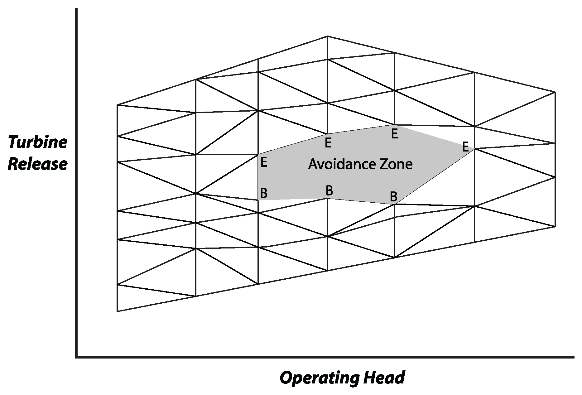
Let us identify the avoidance zone values from the power table in the following way for the algorithm:
• B - the beginning, low flow, of an avoidance zone for a given head
• E - the end, high flow, of an avoidance zone for a given head. If either the maximal or minimal head has a single flow value, then that point is marked E.
Pseudocode for Triangulation
The basic idea is to iterate through the Head values in the (reduced) Unit Power Table, partitioning the vertical space between that head and the next into triangles. In general when deciding which of two potential triangles to create, RiverWare creates the one that has the lesser slope for the upper side.
// Triangulate between each pair of adjacent heads
For H1 = first head to next to last
H2 = next H
// Start with the minimum flow for each head
Q1 = First Q for H1
Q2 = First Q for H2
// At each step increment one of the flows to form a triangle
While (next Q1 != NULL || next Q2 != Null)
// If only Q1 can be incremented or incrementing Q1 leads to a flatter triangle top, increment Q1 and form
// the triangle
If (next Q2 = NULL || next Q1 - Q2 <= next Q2 - Q1)
Create a Triangle with coordinates(H1.Q1, H1.next Q1, H2.Q2)
Q1 = next Q1
Else
Create a Triangle with coordinates(H1.Q1, H2.next Q2, H2.Q2)
Q2 = next Q2
// If the two heads are at an avoidance zone, increment Q past it
If (Q1 is marked B && Q2 is marked B or E)
Q1 = next Q1
If (Q2 is marked B && Q1 is marked B or E)
Q2 = next Q2
If head is specified, then the triangles become line segments, and line segments become points.
Lambda Variables for Convex Combinations of Discrete Operating Points (Triangles)
In the context of optimization, a lambda set is (roughly) a discretization of a continuous space, so RiverWare uses this technique to model the discretization of the power curve domain into triangles. While solvers don’t require it, usually it is assumed that lambda variables are constrained as follows:
0 <= Lambda_subscripts <= 1
Sigma (some subscripts, Lambda_subscripts) = 1
Lambda sets may additionally be constrained to be a specially ordered set of type 1 or 2, aka SOS1 or SOS2. The individual variables in an SOS are ordered and a reference row of weights is associated with each variable. An SOS1 may have at most one value that is nonzero while an SOS 2 may have at most two nonzero values and they must be adjacent. Solvers internally treat these sets as being similar to integer variables with branching to enforce the set conditions. The branching is based on weights in the reference row. The general idea is to calculate a weighted average of the variables using the reference row. The two branches are roughly that either variables on one side of the weighted average are zero or the variables on the other side are zero.
In addition, frequently the individual variables belonging to an SOS1are also binary variables. The variables in a SOS2 are almost always continuous.
Power is a nonlinear function of both flow and head. Hence, when it is discretized, the domain of the function is two-dimensional. The SOS technique can be applied here as well. In this case, a combination of 3 points is used to define flow and head. Alexander Martin has described how to model this case as an SOS type k, where k is 3 in this case (A. Martin, “Approximation of Non-linear functions in Mixed Integer Programming” Workshop on Integer Programming and Continuous Optimization, Chemnitz University of Technology, November 7–9, 2004, www-user.tu-chemnitz.de/~helmberg/workshop04/martin.ppt). Martin then modifies a solver to directly branch on the SOS k, creating separate branches for each region of the domain.
Note: Some solvers have an SOS 3, but this typically does not refer to the same thing as it is used here.
A variant of his method that is compatible with CPLEX and other solvers is used here. The flow and head domains are partitioned into triangles and define a variable for each triangle, Lambda_1. The triangles in an SOS 3 are analogous to the line segments in an SOS 2. The triangulation is described in section 2.7.
The following lambda variables are part of the formulation:
• Lambda_1rut: selection of triangular region r on unit u
This variable binary, technically an SOS k, Lambda_2 is used to implement this functionality. Therefore, there is no need for a reference row and its weights. This variable may represent 2 points instead of 3 if a feasible region is one-dimensional. For example most data sets will contain points with zero flow for several heads, but disallow small flows. Thus, the segment of zero flow between adjacent heads will be a Lambda_1 variable even though it is not a triangle. In theory, there could be a single isolated operating point that would need its own Lambda_1 variable, but this is unlikely in practice.
• Lambda_2h’ut: selection of a triangle with approximate head h’ for unit u.
This is a binary variable, SOS1 for each t: reference row weights are the approximate head (half way between the two head values for the points in the triangle). The set of Lambda_1rut triangles with r in h’ form an SOS1 for each h’,u,t combination. The reference row weights are the average q value of the points in the triangle. In addition the sum is constrained to equal Lambda_2h’ut:
• Lambda_4hut: selection of head h
This is a continuous variable, SOS2 for each u,t: the reference row weights are head.
• Lambda_6hqut: combination of o and q
This is a continuous variable, not an SOS. The data should include q=0 for all possible heads, even those that cannot generate power.
The set of Lambda_6hqut points with the same o form an SOS2 for each h,u,t combination. The reference row weights are the q values.
Defining Constraints
This section presents the constraints which will be introduced into the optimization problem as power-related quantities are encountered in the optimization policy (when the Unit Power method is selected).
Notes on Variables and Notation
All variables are constrained to be positive unless otherwise noted.
Binary Variables
These variables are required to be zero or one, and will be enforced on user inputs in the corresponding slots at the beginning of the run.
• Unit Is Generating (UIGut)
• If the Startup method is selected
– Unit Startup (USUut)
– Unit Shutdown (USDut)
• Lambda 6 variables (Lambda_6put)
Continuous Variables
• If the Shared Penstock Head Loss method is selected,
– PNHt = Net head after losses in the shared penstock
– SPHt = Shared penstock losses
• If the Unit Regulation method is selected,
– RUFhqut = Fraction of possible regulation up at point indexed by hqu being used
– RDFhqut = Fraction of possible regulation down at point indexed by hqu being used
Symbols
The following symbols will be used in the formulation below (see also slot summary table):
• Xp = The X component of point p in a data table (i.e., the value in the column labeled X)
• WQru = turbine flow weighting of triangle r on unit u. Equal to the average of flow on the points r contains.
• WHru = head weighting of unit triangle r on unit u. Equal to the average of head on the points r contains.
• TWMpu = minimum tailwater that allows point Lambda_6put to be feasible
• MinTW = minimum possible tailwater at the plant
• TW = plant tailwater elevation
• QTr = maximum turbine release for triangle r
The following indexes are used:
• h’ = approximate head index for power triangles with their center of mass within a tolerance of the operating
• r = triangle region of the power curve where convex combinations are allowed.
• u = unit index
• t = time
• p = point in a table. E.g., for the Unit Power table each point is a triplet (QT, H, P), so QTp denotes the Flow component of p, Hp denotes the head component, and Pp denotes the Power component. Similarly, the Unit Regulation Table has sextets of (QT,H, RUL,QTUL,RDL, QDL). RULp denotes the Regulation Up Limit, the maximum power generation that can be attained by increasing flow at the specified operating head without passing through an avoidance or cavitation zone. Similarly, RDLp is the Regulation Down Limit, QTUL and QTDL are the flow values associated with these power values.
Sigma indicates capital sigma used for a summation. The arguments following sigma in parenthesis are respectively the indexes to sum over and the expression summed.
Bold typeface for a variable indicates the constraint is a defining constraint for that variable.
The constraints are presented with an unspecified timestep (t) and unit (u). Instantiations will be created during the run only for those units and timesteps which are referenced by the user’s policy.
Unit-level Constraints
1. Unit Is Generating is equivalent to selecting a triangular region above zero flow/generation
“Unit Generation Constraint”
Sigma (r with QTru > 0, Lambda_1rut) = UIGut
2. Unit Start up and Shut down
If the Unit Lumped Cost startup method is selected,
“Unit Startup Constraint”
UIGut – UIGut - 1 = USTu,t – USHu,t
3. Operating Head or Net Head is discretized by Lambda_4
If there is no additional head loss (No Method in the Head Loss category) is selected
“Operating Head Unit Lambda Constraint”
POHt = Sigma (head h in Unit Power Table with unit u, Hhu * Lambda_4hut)
Else If the Shared Penstock Head Loss method is selected
“Net Head Unit Lambda Constraint”
PNHt = Sigma (head h in Unit Power Table with unit u, Hhu * Lambda_4hut)
4. Net Head Definition
If the Shared Penstock Head Loss method is selected:
“Net Head Constraint”
PNHt = OHt - SPHt (Net Head = Operating Head - Shared Penstock Loss)
5. Specified Power – Flow curve from Lambda_6 points
If the Unit Frequency Regulation method is selected:
“Unit Scheduled Mechanical Power Constraint”
USMPut = Sigma (p in Unit Power Table with unit u, Ppu * Lambda_6put)
Else
“Unit Power Constraint”
UPut = Sigma (p in Unit Power Table with unit u, Ppu * Lambda_6put)
If the Unit Frequency Regulation method is selected:
“Unit Scheduled Turbine Release Constraint”
USQTut = Sigma (p in Unit Power Table with unit u, QTpu * Lambda_6put)
Else
“Unit Expected Turbine Release Constraint”
UEQTut = Sigma (p in Unit Power Table with unit u, QTpu * Lambda_6put)
6. Tailwater Limit to Prevent Cavitation
“Tailwater Cavitation Constraint”
TWt - MinTW >= Sigma (p in Unit Power Table with unit u, (TWMpu - MinTW) * Lambda_6put)
Note: TWMpu - MinTW should be 0 for most power points
7. Minimum Power Elevation
if MinPPEu != NaN
“Minimum Power Elevation Constraint”
PEt - MinPE >= (MinPPEu - MinPE) UIGut
8. Power – Flow regulation up equals a fraction of the limit
If the Unit Frequency Regulation method is selected,
“Unit Regulation Up Constraint”
URUut = Sigma (p in Unit Regulation Table with unit u, RULpu * UPRUut)
“Unit Flow Addition for Regulation Constraint
UQARut = Sigma (p in Unit Regulation Table with unit u, QTULpu * UPRUut)
“Unit Regulation Up Lambda_6 Constraint”
For all unit u, for all p in Unit Power Table
UPRUut <= Lambda_6pt
9. Power - Flow regulation down equals a fraction of the limit
If the Unit Frequency Regulation method is selected,
“Unit Regulation Down Constraint”
URDut = Sigma (p in Unit Regulation Table with unit u, RDLpu * UPRDut)
“Unit Flow Reduction for Regulation Constraint
UQRRut = Sigma (p in Unit Regulation Table with unit u, QDLpu * UPRDut)
“Unit Regulation Down Lambda_6 Constraint”
For all unit u, for all p in Unit Regulation Table
UPRDut <= Lambda_6put
10. Two-sided regulation tied to regulation up and down
If the Unit Frequency Regulation method is selected,
“Two-sided Regulation Limited by Regulation Up”
UTSRut <= URUut
“Two-sided Regulation Limited by Regulation Down”
UTSRut <= URDut
11. Expected power and flow after regulating
If the Unit Frequency Regulation method is selected,
“Expected Unit Power Constraint”
UPut = USMPut + URUut/2 - URDut/2
12. Unit Operating Costs
If the Unit Frequency Regulation method is selected,
“Unit Operating Cost Constraint”
UOCut = timestepHRS * UOCPR * (RUut + RDut)
13. Unit Startup Costs
Unit Startup Cost is replaced using the following definition:
USCut = Unit Startup Cost Table u * USTut
14. Unit Priority Constraints
Ordering the units will considerably reduce the search space, particularly if the some of the units are identical. In addition, this is often an operating policy.
For unit i with a higher priority than unit j:
“Precedence Constraint”
UIGit > UIGjt
Defining Constraints for Lambda Variables
1. Lambda1 Unity Constraint
Sigma(r with unit u, Lambda_1rut) = 1
2. Lambda6 Unity Constraint
Sigma(p in Unit Power Table with unit u, Lambda_6put) = 1
Note: The Lambda_2 unity constraint is omitted because it is implied by Lamba_1, and the Lambda_4 unity constraint because it is implied by Lambda_6.
3. Lamba1 Definition Constraint
For all h’:
Sigma (r in h’, Lambda_1rut ) = Lambda_2h’t
4. Lambda 2 Definition Constraint
For each Lambda_4 variable from the triangles, the sum of the adjacent Lambda_4 variables must be greater than the Lambda_2 variable:
For all h’:
Sigma (h adjacent to h’, Lambda_4hut) >= Lambda_2h’ut
5. Triangle Definition Constraint
The sum of the use of the points of a triangle must be greater than the triangle variable:
For all r:
Sigma (p in r, Lambda_6put) >= Lambda_1rut
6. Lambda 6 Definition Constraint - the sum is constrained to equal Lambda_4hut
For all h:
Sigma (p with Head value = h, Lambda_6put) = Lambda_4hut
Unit/Plant Relationship Constraints
Any plant variable, PVx, where x represents the appropriate subscripts is defined by the sum of the unit variables, Vux, indexed by unit u and x. Plant variables are only created if they are used directly or indirectly by policy. Thus, the defining constraint is as follows:
“Plant Unit V Constraint”
PVx = Sigma(u,Vux)
Redefining Existing Plant-level Linearizations
The modeling of power will be more accurate when lambda variables and SOS sets are used to replace the plant level linearization of pool elevation and tailwater. Both of these affect operating head. This has been temporarily postponed until a potential problem is addressed: the associated lambda variables might be frozen by an objective solved using linear programming before it reaches the power objective. If this were to occur, the intended model for integer programming would be disrupted. This is more likely to be a problem for pool elevation than tailwater because pool elevation is important for non-power policy, whereas tailwater is usually only important for power. Moreover, the error in existing methods is larger for tailwater than pool elevation. For these reasons, it is more likely beneficial to change the modeling of tailwater.
The pool elevation constraints are:
“Pool Elevation Lambda Constraint”
PEt = Sigma(p in Elevation Volume Table, PEp * Lambda_7st)
“Pool Elevation Lambda Storage Constraint”
St = Sigma(p in Elevation Volume Table, SEp * Lambda_7st)
“Pool Elevation Lambda Unity Constraint”
Sigma(p in Elevation Volume Table, Lambda_7pt) = 1
Lambda_7 is an SOS2
If the tailwater method is optTWStageFlowLookupTable, the tailwater constraints define tailwater, outflow, and tailwater base value in terms of Lambda_8 points directly or indirectly in terms of Lambda_9 and Lambda_10:
“Tailwater Stage Flow Lambda Constraint”
TWt = Sigma(p in Stage Flow Tailwater Table, TWp * Lambda_8pt)
“Tailwater Stage Flow Lambda Flow Constraint”
Qt = Sigma(flow q in Stage Flow Tailwater Table, Qq * Lambda_10qt)
“Tailwater Stage Flow Lambda Base Value Constraint”
TWBVt = Sigma(tailwater base value v in Stage Flow Tailwater Table, TWBVv * Lambda_9vt)
“Tailwater Stage Flow Lambda Unity Constraint”
Sigma(p in Stage Flow Tailwater Table, Lambda_8pt) = 1
“Tailwater Stage Flow Lambda Base Value Lambda Constraint”
For all v:
Sigma (p in Stage Flow Tailwater Table with tailwater base value = v, Lambda_8pt) = Lambda_9vt
“Tailwater Stage Flow Lambda Flow Lambda Constraint”
For all q:
Sigma (p in Stage Flow Tailwater Table with outflow = q, Lambda_8pt) = Lambda_10qt
Lambda8 is an SOSk implemented by making Lambda_9 and lambda_10 SOS2s. An alternative implementation would be triangles as used for power.
If the tailwater method is optTWBaseValuePlusLookupTable, the new tailwater constraints define temp tailwater lookup and outflow in terms of Lambda_11:
“Tailwater Lookup Lambda Constraint”
TWLt = Sigma(f, TWTf * Lambda_11ft)
“Tailwater Lookup Lambda Flow Constraint”
Qt = Sigma(f, TWQf * Lambda_11ft)
“Tailwater Lookup Unity Constraint”
Sigma(f, Lambda_11ft) = 1
Lambda_11 is an SOS2
For this method, the existing tailwater constraint is retained:
TWt = (TWBVt + TWBVt-1) / 2 + TWLt
Thermal Object
The thermal object has a number of multi-slots that are potential variables in an optimization problem. These multi-slots typically represent the system wide total of individual reservoir values that are linked to these slots. Equations for these sums are added automatically if a policy either directly or indirectly references one of the thermal object multi-slots.
Many of the existing variables and definitions are already on the thermal object. In addition, to the existing equations, the following new equations will be added.
System Regulation Up is greater than the sum of Block Regulation Up variables:
SRUt * timestepHRS >= Sigma(b, BRUbt)
The Regulation Up Value equals the sum of the value of the Block Regulation Up variables:
RUV = Sigma(b, RUBCb * BRUbt)
System Regulation Down is greater than the sum of Block Regulation Down variables:
SRDt * timestepHRS >= Sigma(b, BRDbt)
The Regulation Down Value equals the sum of the value of the Block Regulation Down variables:
RDV = Sigma(b, RDBCb * BRDbt)
Revised: 08/02/2021