
Routing
The Routing method determines how the flow is calculated. It can also effect what dispatch methods and user categories are available for use. Some of the Routing methods may only solve downstream (for outflow), while others may solve either upstream or downstream.
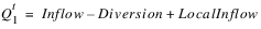
No Routing is the default method for this category. This method involves a simple mass balance. It triggers the selection of dispatch methods that perform the actual calculations. It is the only method for which local Inflow may be calculated.
The calculations are executed by the dispatch methods, Solve given Outflow, No Routing; Solve given Inflow, No Routing; and Solve given Inflow, Outflow, No Routing.
Slots Specific to This Method
Return Flow
Type: Series
Units: FLOW
Description: return flow into the reach
Information: Enters at the bottom of the reach (that is, it is added directly to the outflow calculated by the method).
I/O: Optional; if not input and not linked, it is set to zero.
Links: May be linked to the Return Flow slot on any object, the Outflow slot on a Groundwater Storage object, the Excess GW Outflow slot on the Groundwater Storage object, or the Surface Return Flow slot on a WaterUser.
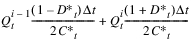
Inflows are lagged by a specified time to calculate outflows. This method can be solved upstream or downstream and therefore causes dispatching with either a known inflow or a known outflow. The lagtime can be any length of time.
Slots Specific to This Method
LagTime
Type: Scalar
Units: TIME
Description: lagtime or travel time of a flow change through the reach
Information:
I/O: Required input
Links: Not linkable
Method Details
Following is a sample equation for Outflow:

where (-1) means the value at the previous timestep.
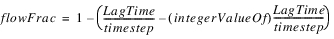
Following is the equation for flow fraction:
This method can also solve for inflow, given outflow.
Note: It is possible to set up a combination of input values for inflow and outflow that do not match. This will cause an error. An error will also result if the timestep is 1 Month and the Lag Time is not in months, or if the timestep is not 1 Month and the Lag Time is in months.
Behaves similarly to Time Lag routing except that the Lag Time is allowed to vary as a function of the day of the year and the flow rate. This method can only solve downstream.
Slots Specific to This Method
Return Flow
Type: Series
Units: FLOW
Description: return flow into the reach
Information: Enters at the bottom of the reach (that is, it is added directly to the outflow calculated by the method).
I/O: Optional; if not input and not linked, it is set to zero.
Links: May be linked to the Return Flow slot on any object, the Outflow slot on a Groundwater Storage object, the Excess GW Outflow slot on the Groundwater Storage object, or the Surface Return Flow slot on a WaterUser.
Variable Lag Time
Type: Series
Units: TIME
Description: value of the Lag Time interpolated from the Variable LagTime Table.
Information:
I/O: Output only
Links: Not linkable
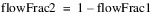
Variable LagTime Table
Type: Table
Units: TIME VS. Flow VS. TIME
Description: a table relating the day of the year, flow rate, and the lag time
Information: Data must be entered in blocks of increasing flow for each given day for the interpolation method to work correctly. January 1 is represented by a 1, February 1 as 32, and so on. Following is an example table.
Day of Year | Flow Rate | Lag Time |
|---|---|---|
1 | 500 | 1.0 |
1 | 550 | .9 |
1 | 600 | .8 |
32 | 500 | 2.0 |
32 | 550 | 1.7 |
32 | 600 | 1.5 |
60 | 500 | 2.1 |
60 | 550 | 1.9 |
60 | 600 | 1.6 |
I/O: Required input
Links: Not linkable
Method Details
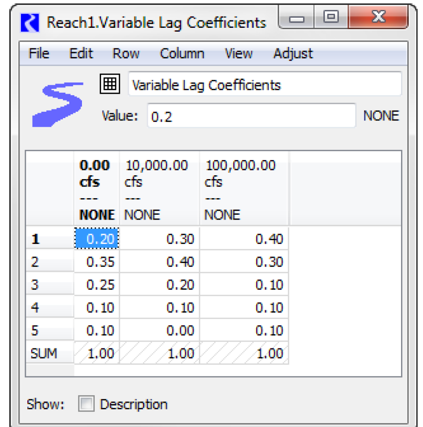
This method executes when the Inflow is known for the current timestep. The Inflow value is then used to calculate the Variable Lag Time. Outflow values can then be solved for at the timesteps corresponding to the Variable Lag Time. Following is a sample calculation:


where flowFrac1 and flowFrac2 to are calculated by the following equations:

In these equations, the integer value of a number means that the number is truncated after the decimal point with no rounding.
Since the lag time can vary with every timestep, it possible that more the one Inflow can contribute to a particular Outflow. Return Flow and Total Gain Loss can then be added to the calculated Outflow value.
This function solves for the outflow from a reach given inflow.
Slots Specific to This Method
Lag Coeff
Type: Table
Units: NO UNITS
Description: impulse response coefficients
Information:
I/O: Required input
Links: Not linkable
Num. of Coeff
Type: Scalar
Units: NO UNITS
Description: number of impulse response coefficients
Information:
I/O: Required input
Links: Not linkable
Return Flow
Type: Series
Units: FLOW
Description: return flow into the reach
Information: Enters at the bottom of the reach (that is, it is added directly to the outflow calculated by the method).
I/O: Optional; if not input and not linked, it is set to zero.
Links: May be linked to the Return Flow slot on any object, the Outflow slot on a Groundwater Storage object, the Excess GW Outflow slot on the Groundwater Storage object, or the Surface Return Flow slot on a WaterUser.
Method Details
There must be the same number of values in the Lag Coeff table as the value given in Num of Coeff in order to successfully dispatch at any timestep. If any needed value is invalid, an error will occur, and the run will stop.
The general equation for this method is as follows:

Note: If a new value is set for Inflow at a given timestep, the reach will re-dispatch to solve for a new Outflow at that timestep only. It will not, in general, re-solve for Outflow at every timestep that is affected by the new Inflow. For example, say the Outflow at timestep t is a function of the Inflow at t, t - 1, and t - 2. If a new Inflow value is set at timestep t - 2, the reach will redispatch and solve for a new Outflow at t - 2, but it will not re-dispatch at timesteps t - 1 and t. Thus the final Outflow values at t - 1 and t will not correspond to the updated Inflow value at t - 2. If this type of redispatching across multiple timesteps is required, the Step Response routing method should be used; see Step Response.
The step response method is a simple routing method that computes outflow for the current timestep and future timesteps given inflow values. The total number of outflows computed will be equal to the number of lag coefficients. The outflow will be computed as the sum of the routed inflows plus whatever sources or sinks may be available.
Slots Specific to This Method
Return Flow
Type: Series
Units: Flow
Description: return flow into the reach
Information: Enters at the bottom of the reach (that is, it is added directly to the outflow calculated by the method).
I/O: Optional; if not input and not linked, it is set to zero
Links: May be linked to the Return Flow slot on any object, the Outflow slot on a Groundwater Storage object, the Excess GW Outflow slot on the Groundwater Storage object, or the Surface Return Flow slot on a WaterUser.
Lag Coeff
Type: Table
Units: No Units
Description: step response coefficients
Information: The number of Lag Coefficients must be equal to the value in the Num. of Coeff slot.
I/O: Required input
Links: Not linkable
Num. of Coeff
Type: Scalar Slot
Units: No Units
Description: number of step response coefficients
I/O: Required input
Links: Not linkable
Method Details
The general calculations for this method are very similar to the Impulse Response routing method.
1. First, the outflow for the current timestep is calculated.

2. The method will then move on to the first future outflow. At this stage, outflow will be computed using the same equation only now, t will be incremented to t+1, t-1 incremented to t, and so on. The total Gain Loss term will be the Total Gain Loss for timestep t+1.
3. In the situation where the method is looking for an inflow for a timestep that is actually past the current timestep and this value is not valid, this inflow will be assumed to be zero. If the inflow is not valid for a previous timestep, the calculation will exit and the method will move on to the next future timestep.
The Variable Step Response method is a variation of the Step Response routing method that computes outflow for the current timestep and future timesteps given inflow values. The total number of outflows computed will be equal to the number of lag coefficients. The outflow will be computed as the sum of the routed inflows plus whatever sources or sinks may be available. In the Step Response method, a single set of lag coefficients is used. In the Variable Step Response method, multiple sets of lag coefficients are used dependent on the inflows to the reach.
Slots Specific to This Method
Return Flow
Type: Series
Units: Flow
Description: return flow into the reach
Information: Enters at the bottom of the reach (that is, it is added directly to the outflow calculated by the method).
I/O: Optional; if not input and not linked, it is set to zero
Links: May be linked to the Return Flow slot on any object, the Outflow slot on a Groundwater Storage object, the Excess GW Outflow slot on the Groundwater Storage object, or the Surface Return Flow slot on a WaterUser.
Variable Lag Coefficients
Type: Table Slot
Units: Column Map Values - Flow, Table values - No Units
Description: A table defining the step response coefficients for each inflow threshold is shown.
Information: This table has a column map, which means that each column has an associated numerical value (with units). This numerical value is displayed as the column label.
Columns are added and deleted from this table using the Column menu with the following options: Set Number of Columns, Append Column, Delete Column and Delete Last Column.
User units, scale, type, and precision for the column map (that is, the column heading values) are defined in the unit scheme for Flow unit types. Column map values are set from the Column, Set Column Value menu option.
When a column value is changed, the columns reorder to ensure the column values are increasing, from left to right.
The sum of coefficients in each column should equal 1.0. This can be verified by adding a summary row at the bottom of the table by selecting View, then Show Column Sum Row.
When used in the Variable Step Response method, the column map values are used as a stair-step lookup. For example, an Inflow of 500cfs uses the first column; an inflow of 10,000cfs uses the second column; and an inflow of 120,000cfs uses the third column. Therefore, the column map values need not bound the highest expected flows; flows greater than the largest column map value use the right-most column.
Note: The left-most set of coefficients should represent the minimum flow in the reach.
I/O: Required input
Links: Not linkable
Method Details
This Routing method is executed from the Solve given Inflow dispatch method; that is, it only solves for the Outflow given the Inflows, not vice versa.
Note: Local Inflows are added to the top of the reach and are routed with the Inflows.
In the following, Inflow refers to the sum of the Inflow and Local Inflow slot. The variable ncoeff is the number of rows in the Variable Lag Coefficients slot. The outflows will be calculated using the following algorithm:
For each t from (t = 0 that is, current timestep) to (t = current timestep + (ncoeff - 1))

End for
Each C coefficient is selected from the appropriate column of the Variable Lag Coefficients slot based on the value of the Inflow with which it is multiplied. For a particular evaluation of the equation, the sum of the coefficients does not necessarily equal 1.0. But, mass is preserved over time. Using the above sample table, if the Inflow at the current timestep t, is 12,000cfs and the Inflow at t-1 is 8,000cfs, C0 is 0.30 and C1 is 0.35 using the above table.
If the method is looking for an inflow for a timestep that is actually past the current timestep and the value is not valid, this inflow will be assumed to be zero. If the inflow is not valid for a previous timestep, the calculation will exit the method without calculating an outflow, post a warning message, and move on to the next timestep.
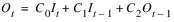
The Muskingum method is a simple storage routing method that solves for the propagation of flow waves based on a lag time and attenuation factor.
Note: This method must have Inflow and Outflow known at the timestep before the first routing timestep.
The Muskingum method only allows for one routing segment, but allows for Local Inflows, Diversions, and Return Flow. The Muskingum with Segments method (described next) allows for multiple segments, but no Diversions, Local Inflows, or Return Flows.
Slots Specific to This Method
Return Flow
Type: Series
Units: FLOW
Description: return flow into the reach
Information: Enters at the bottom of the reach (that is, it is added directly to the outflow calculated by the method).
I/O: Optional; if not input and not linked, it is set to zero.
Links: May be linked to the Return Flow slot on any object, the Outflow slot on a Groundwater Storage object, the Excess GW Outflow slot on the Groundwater Storage object, or the Surface Return Flow slot on a WaterUser.
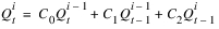
Method Details
Following is the general equation for this method:

where outflow and outflow(-1) are the current and previous outflows respectively as with inflow and inflow(-1).
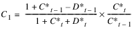
Note: The routing parameters (either directly as C0,C1,and C2 or as K and X) are specified by the Routing Parameters category.
This routing method is called from the Solve given Inflow dispatch method. That is, when Muskingum with Segments is selected, the only dispatch method is Solve given Inflow. This routing method also includes optional Bank Storage, Gain Loss, Outflow Adjust, and Stage calculations.
Note: All these calculations occur after the routing has occurred, based on the routed flow.
Slots Specific to This Method
Number of Segments in Reach
Type: Scalar
Units: None
Description: Number of segments
Information: This parameter determines the number of columns in the Segment Outflow table. In the equations below, the number of segments is represented by the variable n.
I/O: Required input
Links: Not linkable
Outflow by Segment
Type: Agg Series
Units: FLOW
Description: Segment outflow. The segments are numbered upstream to downstream. The Outflow to one segment is the inflow to the next segment.
Information: The outflow from the reach is the outflow from the last segment. The columns in this slot will be resized to the number of segments input by the user, and the number of rows will be the number of timesteps in the run. At the beginning of the run, if the initial timestep Outflow by Segment is not known, the Outflow by Segment is set to the Reach Inflow or Outflow, if known.
Information: Input at Initial timestep, Output at other timesteps
I/O: Output only
Links: Not linkable
Method Details
Following is the general equation for this method:

where Outflow and Outflow(-1) are the current and previous outflows respectively as with Inflow and Inflow(‑1).
You can further discretize the reach into n sub-reaches for better control over attenuation.
Note: The routing parameters (either directly as C0,C1,and C2 or as K and X) are specified by the Routing Parameters category and the same parameters are used for each segment in the reach.
First, the method checks the following:
1. The current timestep’s inflow is checked. It should be known or the dispatch method would not have been called.
2. If the previous Inflow is not known, the method exits and waits.
3. The Outflow by Segment from the previous timestep is checked for validity. If they are all valid from previous solutions, they are used directly and the method continues. If any of the Outflow by Segment are not valid, the following checks are made:
a. If the Outflow is not known and the last Outflow by Segment is known, then Outflow is set to that value. All other Outflow by Segments are also set to that value.
b. If the Outflow is not known, Outflow and each Outflow by Segment is set equal to the Inflow and the routing method exits. This scenario can occur the first time the reach dispatches. This situation is used when you would like the initial Outflow = Inflow.
c. If the Outflow is known (input or set by a rule), each Outflow by Segment is set equal to the Outflow and the method exits. This scenario can occur the first time the reach dispatches and achieves the need where initial Outflow is specified.
4. Then, the method executes the selected method in the Routing Parameters category to determine the C0,C1,and C2 parameters. These C0,C1,and C2 are used by each segment in the reach.
5. Next, the method sets up arrays of the variables I and O with the known information. The arrays have 2 rows (timesteps) and n columns (segments).
Note: I(t, 1) = Inflow. Table 23.1 shows the array with the variables. Those next to each other are set to the same value, for example O(t-1,2) = I(t-1,3).
Timestep | Reach | Segment 1 | Segment 2 | Segment3 | Reach | |||
|---|---|---|---|---|---|---|---|---|
t-1 | Inflow(t-1) | I(t-1,1) | O(t-1,1) | I(t-1,2) | O(t-1,2) | I(t-1,3) | O(t-1,3) | Outflow(t-1) |
t | Inflow(t) | I(t,1) | O(t,1) | I(t,2) | O(t,2) | I(t,3) | O(t,3) | Outflow(t) |
6. Next, loop over each segment and compute the outflow for each segment upstream to downstream:
For (j=1 to Number of Segments)
Compute the Outflow from this segment

Set the inflow value for the next segment, I(t,j+1) = O(t,j)
End For
7. Set the slot Outflow by Segment[t,j] to the values stored in the O array.
8. Execute Reach Bank Storage and Reach GainLoss method using the routed flow (Outflow in the last segment)
9. Set the Reach Outflow equal to the last segment’s outflow plus Bank Storage Return flow plus Total Gain Loss.
10. Execute the selected Outflow Adjustment method and reset Outflow if necessary
This hydraulic routing method is a finite difference solution of the kinematic wave simplification to the St. Venant Equations. It requires a numerical grid to be specified by the user. The numerical approximation tends to result in a negative mass balance error (reaches lose water) in test models. To reduce the mass balance error, CADSWES recommends using the Kinematic Improved method; see Kinematic Improved.
Slots Specific to This Method
Delta X Computational Element Length
Type: Scalar
Units: LENGTH
Description: size of the x discretization
Information: This slot must be smaller than the Reach Length
I/O: Required input
Links: Not linkable
Distributed Depth Output
Type: Table Series
Units: LENGTH
Description: depth at upstream end of each element
Information: This value is calculated by the selected Depth to Flow method after calculating the Distributed Flow Output for the current segment at the current timestep.
I/O: Output only; this is a temporary slot that is not saved in the model file.
Links: Not linkable
Distributed Celerity Output
Type: Table Series
Units: VELOCITY
Description: celerity(wave speed) at upstream end of each elements
Information: This value is calculated by the selected Depth to Flow method after calculating the Distributed Flow Output for the current segment at the current timestep. Celerity from the previous timestep is used to calculate Distributed Flow Output at the current timestep.
I/O: Output only; this is a temporary slot that is not saved in the model file.
Links: Not linkable
Distributed Flow Output
Type: Table Series
Units: FLOW
Description: inflow value at the upstream end of each element
Information: This value is calculated using Celerity from the previous timestep at the current element according to the equation in step 1 below.
I/O: Output only; this is a temporary slot that is not saved in the model file.
Links: Not linkable
Distributed TopWidth Output
Type: Table Series
Units: LENGTH
Description: width of top of water surface
Information: This value is calculated by the selected Depth to Flow method after calculating the Distributed Flow Output for the current segment at the current timestep.
I/O: Output only; this is a temporary slot that is not saved in the model file.
Links: Not linkable
Distributed Velocity Output
Type: Table Series
Units: VELOCITY
Description: velocity at upstream end of each element
Information: This value is calculated by the selected Depth to Flow method after calculating the Distributed Flow Output for the current segment at the current timestep.
I/O: Output only; this is a temporary slot that is not saved in the model file.
Links: Not linkable
Distributed Volume Output
Type: Table Series
Units: VOLUME
Description: volume contained in each element
Information: The volume in each segment is calculated as follows. Because this routing method is a numerical approximation, the segment outflow values will contain numerical error. This numerical error will accumulate in the Distributed Volume Output calculations. Thus this slot can be used to evaluate the overall mass balance error when using the Kinematic method.

I/O: Output only; this is a temporary slot that is not saved in the model file.
Links: Not linkable
Distributed Xsectional Area Output
Type: Table Series
Units: AREA
Description: area at upstream end of each element
Information: This value is calculated by the selected Depth to Flow method after calculating the Distributed Flow Output for the current segment at the current timestep.
I/O: Output only; this is a temporary slot that is not saved in the model file.
Links: Not linkable
Numerical Parameters Output
Type: Table
Units: VARIOUS
Description: Columns describing grid and Courant number of each element for the current timestep
Information: The rows of this table store the value of the Courant number with respect to distance. The number of rows used is based on the discretization parameters defined by the user, Number of each Length/Delta X. The number of rows in this table is currently limited to 500; therefore, the number of computational elements for each reach must not be greater than 500; that is, Delta X must not be less than Reach Length/500. The first two columns are computed at the beginning of run. The Courant number is computed and updated every time the reach dispatches and routes the flow.
I/O: Output only
Links: Not linkable
Reach Length
Type: Scalar
Units: LENGTH
Description: total length of the reach, from upstream to downstream.
Information: This slot must be larger than Delta X
I/O: Required input
Links: Not linkable
Return Flow
Type: Series
Units: FLOW
Description: return flow into the reach
Information: Enters at the bottom of the reach (that is, it is added directly to the outflow calculated by the method).
I/O: Optional; if not input and not linked, it is set to zero.
Links: May be linked to the Return Flow slot on any object, the Outflow slot on a Groundwater Storage object, the Excess GW Outflow slot on the Groundwater Storage object, or the Surface Return Flow slot on a WaterUser.
Method Details
The solution is a nonlinear numerical approximation to the following continuity and momentum equations.
Continuity 
Momentum 
For this numerical solution, accuracy increases as the Courant number approaches unity and decreases as the Courant number diverges from unity. The Courant number for each numerical grid section for the current timestep can be observed in the Numerical Parameters Output under the column labeled Courant. The Courant number is calculated as follows:

where c = wave celerity [L/T],  t = routing time step[T], and
  x = spatial step size[L].
t = routing time step[T], and x = spatial step size[L].This hydraulic routing method also requires the user to select from another category of user selectable methods, Depth to Flow. The inputs for these methods are described under that user method category.
In the following method, a superscript refers to the timestep, and a subscript refers to the spatial location (element number) within the reach, upstream to downstream.
Note: This method is restricted to using a non-zero Inflow for the initial timestep. The Kinematic Improved method does not have this restriction; see Kinematic Improved.
1. At the start of the run this method sets all columns of the Distributed Flow Output at the initial timestep (Start Timestep - 1) equal to the initial Reach Inflow (that is, the flow is the same at every element). It then calls the selected Depth to Flow method to calculate all flow parameters for each element at the initial timestep.
2. For each timestep within the run, it first sets the flow for the first element, as follows:

3. If Diversion or Local Inflow are not used, they are set to zero.
4. Then the selected Depth to Flow method is called calculate all flow parameter values for the first element using  . The values are set in the first column of the Distributed Output table series slots.
. The values are set in the first column of the Distributed Output table series slots.5. The method then loops over all remaining elements in the reach, upstream to downstream, to carry out the finite difference approximation in the following steps.
a. Calculate the flow in the given element using the finite difference approximation of the kinematic wave simplification to the St. Venant Equations, which has the following form:
(This equation is a rearrangement of equation 9.6.6 in Chow et. al., 19881 with a small modification to the calculation of celerity.)
b. Call the selected Depth to Flow method to calculate flow parameters using  . The values are set in the Distributed Output table series slots. The primary value returned is the celerity (wave speed),
  .
.
. The values are set in the Distributed Output table series slots. The primary value returned is the celerity (wave speed), .c. Calculate the Distributed Volume Output, the volume of water within the element, as follows:

6. After calculating flow at the final element, all gains, losses and Return Flow are added to the final element flow to give the total Reach Outflow.
This hydraulic routing method is a finite difference solution of the kinematic wave simplification to the St. Venant Equations. It requires a numerical grid to be specified by the user. The Kinematic Improved method is very similar to the Kinematic method. The only difference is in the flow value used to calculate celerity and other distributed output values for each element in the reach as detailed below. This formulation allows for a smaller Delta X Computational Element Length, which in turn reduces overall mass balance error when compared to the Kinematic method.
Slots Specific to This Method
Delta X Computational Element Length
Type: Scalar
Units: LENGTH
Description: size of the x discretization
Information: This slot must be smaller than the Reach Length
I/O: Required input
Links: Not linkable
Distributed Depth Output
Type: Table Series
Units: LENGTH
Description: depth at upstream end of each element
Information: This value is calculated by the selected Depth to Flow method using the average of the previous timestep flow at the current element and the current timestep flow at the upstream element.
I/O: Output only; this is a temporary slot that is not saved in the model file.
Links: Not linkable
Distributed Celerity Output
Type: Table Series
Units: VELOCITY
Description: celerity(wave speed) at upstream end of each elements
Information: This value is calculated by the selected Depth to Flow method using the average of the previous timestep flow at the current element and the current timestep flow at the upstream element.
I/O: Output only; this is a temporary slot that is not saved in the model file.
Links: Not linkable
Distributed Flow Output
Type: Table Series
Units: FLOW
Description: inflow value at the upstream end of each element
Information:
I/O: Output only; this is a temporary slot that is not saved in the model file.
Links: Not linkable
Distributed TopWidth Output
Type: Table Series
Units: LENGTH
Description: width of top of water surface
Information: This value is calculated by the selected Depth to Flow method using the average of the previous timestep flow at the current element and the current timestep flow at the upstream element.
I/O: Output only; this is a temporary slot that is not saved in the model file.
Links: Not linkable
Distributed Velocity Output
Type: Table Series
Units: VELOCITY
Description: velocity at upstream end of each element
Information: This value is calculated by the selected Depth to Flow method using the average of the previous timestep flow at the current element and the current timestep flow at the upstream element.
I/O: Output only; this is a temporary slot that is not saved in the model file.
Links: Not linkable
Distributed Volume Output
Type: Table Series
Units: VOLUME
Description: volume contained in each element
Information: The volume in each segment is calculated as follows. Because this routing method is a numerical approximation, the segment outflow values will contain numerical error. This numerical error will accumulate in the Distributed Volume Output calculations. Thus this slot can be used to evaluate the overall mass balance error when using the Kinematic Improved method. The mass balance error can be reduced by reducing the size of Delta X Computational Length.

I/O: Output only; this is a temporary slot that is not saved in the model file.
Links: Not linkable
Distributed Xsectional Area Output
Type: Table Series
Units: AREA
Description: area at upstream end of each element
Information: This value is calculated by the selected Depth to Flow method using the average of the previous timestep flow at the current element and the current timestep flow at the upstream element.
I/O: Output only; this is a temporary slot that is not saved in the model file.
Links: Not linkable
Numerical Parameters Output
Type: Table
Units: VARIOUS
Description: Columns describing grid and Courant number of each element for the current timestep
Information: The rows of this table store the value of the Courant number with respect to distance. The number of rows used is based on the discretization parameters defined by the user, Number of each Length/Delta X. The number of rows in this table is currently limited to 500; therefore, the number of computational elements for each reach must not be greater than 500; that is, Delta X must not be less than Reach Length/500. The first two columns are computed at the beginning of run. The Courant number is computed and updated every time the reach dispatches and routes the flow.
I/O: Output only
Links: Not linkable
Reach Length
Type: Scalar
Units: LENGTH
Description: total length of the reach, from upstream to downstream.
Information: This slot must be larger than Delta X
I/O: Required input
Links: Not linkable
Return Flow
Type: Series
Units: FLOW
Description: return flow into the reach
Information: Enters at the bottom of the reach (that is, it is added directly to the outflow calculated by the method).
I/O: Optional; if not input and not linked, it is set to zero.
Links: May be linked to the Return Flow slot on any object, the Outflow slot on a Groundwater Storage object, the Excess GW Outflow slot on the Groundwater Storage object, or the Surface Return Flow slot on a WaterUser.
Background
The solution is a nonlinear numerical approximation to the following continuity and momentum equations.
Continuity

Momentum

For this numerical solution, the total mass balance error will decrease as the Delta X Computational Element Length ( x) decreases (number of segments increases). Decreasing
  x will reduce the dispersion in the numerical solution, resulting in higher peaks and lower valleys in the Reach Outflow. Decreasing
  x will also increase the Courant number. The Courant number for each numerical grid section for the current timestep can be observed in the Numerical Parameters Output under the column labeled Courant. The Courant number is calculated as follows:
x) decreases (number of segments increases). Decreasing x will reduce the dispersion in the numerical solution, resulting in higher peaks and lower valleys in the Reach Outflow. Decreasing x will also increase the Courant number. The Courant number for each numerical grid section for the current timestep can be observed in the Numerical Parameters Output under the column labeled Courant. The Courant number is calculated as follows:
where c = wave celerity [L/T],  t = routing time step[T], and
  x = spatial step size[L].
t = routing time step[T], and x = spatial step size[L].This hydraulic routing method also requires the user to select from another category of user selectable methods, Depth to Flow. The inputs for these methods are described under that user method category.
In the method description below, a superscript refers to the timestep, and a subscript refers to the spatial location (element number) within the reach, upstream to downstream.
Method Details
At the start of the run this method sets all columns of the Distributed Flow Output at the initial timestep (Start Timestep - 1) equal to the initial Reach Inflow (that is, the flow is the same at every element). It then calls the selected Depth to Flow method to calculate all flow parameters for each element at the initial timestep.
For each timestep within the run, it first sets the flow for the first element, as follows:
If Diversion or Local Inflow are not used, they are set to zero.
Then the selected Depth to Flow method is called calculate all flow parameter values for the first element using  . The values are set in the first columns of the Distributed Output table series slots.
. The values are set in the first columns of the Distributed Output table series slots.The method then loops over all remaining elements in the reach, upstream to downstream, to carry out the finite difference approximation in the following steps.
a. Calculate the temporary flow value to use for flow parameter calculations.
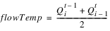
b. Call the selected Depth to Flow method to calculate flow parameters using flowTemp. The values are set in the Distributed Output table series slots. The primary value returned is the celerity (wave speed),  .
.
.c. Calculate the flow in the given element using the finite difference approximation. This finite difference scheme is an implicit backward difference solution of the kinematic wave simplification to the St. Venant Equations and has the following form:
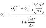
(This equation is a rearrangement of equation 9.6.6 in Chow et. al., 19882. Celerity is substituted using equation 9.3.11.)
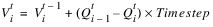
d. Calculate the Distributed Volume Output, the volume of water within the element, as follows:
After calculating flow at the final element, all gains, losses and Return Flow are added to the final element flow to give the total Reach Outflow.
This hydraulic routing method uses the Muskingum routing equation, but with X and K coefficients that are physically based, as an approximation to the diffusive flow equations.
Slots Specific to This Method
Delta X Computational Element Length
Type: Scalar
Units: LENGTH
Description: size of the x discretization
Information: This slot is determined by the method, while it is input by the user for the other hydraulic routing methods.
I/O: Output only
Links: Not linkable
Distributed Celerity Output
Type: Table Series
Units: VELOCITY
Description: celerity(wave speed) at each elements
Information: The value displayed in each row is the value for the last incremental timestep for each run timestep.
I/O: Output only; this is a temporary slot that is not saved in the model file.
Links: Not linkable
Distributed Depth Output
Type: Table Series
Units: LENGTH
Description: depth of each element
Information: The value displayed in each row is the value for the last incremental timestep for each run timestep.
I/O: Output only; this is a temporary slot that is not saved in the model file.
Links: Not linkable
Distributed Flow Output
Type: Table Series
Units: FLOW
Description: flow value of each element
Information: The 0th column represents the flow to be routed (Inflow + Local Inflow - Diversion). The last column represents the routed flow and is copied to the outflow. This is actually the flow for the last incremental timestep and is NOT an average over the timestep.
Note: In the iteration, the method uses the current (t) and next timestep (t+1) rows to store the previous and current values: current row = previous incremental timestep, next row = current incremental timestep. At the end of each incremental timestep, the value is copied from the next timestep’s row to the current timestep’s row. The only effect visible to the user of this iteration mechanism is that the last row of the table is the same as the last minus one row; the last row is beyond the end of the run and can be ignored.
I/O: Output only; this is a temporary slot that is not saved in the model file.
Links: Not linkable
Distributed MuskingumCunge Output
Type: Table
Units: VARIOUS
Description: holds output parameters of routing method.
Information: C0, C1, C2 are all reported here for the current timestep, along with D, C+D, X and K.
I/O: Output only.
Links: Not linkable
Distributed TopWidth Output
Type: Table Series
Units: LENGTH
Description: width of top of water surface
Information: The value displayed in each row is the value for the last incremental timestep for each run timestep.
I/O: Output only; this is a temporary slot that is not saved in the model file.
Links: Not linkable
Distributed Velocity Output
Type: Table Series
Units: VELOCITY
Description: velocity of each element
Information: The value displayed in each row is the value for the last incremental timestep for each run timestep.
I/O: Output only; this is a temporary slot that is not saved in the model file.
Links: Not linkable
Distributed Volume Output
Type: Table Series
Units: VOLUME
Description: volume contained in each element
Information: The value displayed in each row is the value for the last incremental timestep for each run timestep.
I/O: Output only; this is a temporary slot that is not saved in the model file.
Links: Not linkable
Distributed Xsectional Area Output
Type: Table Series
Units: AREA
Description: area of each element
Information: The value displayed in each row is the value for the last incremental timestep for each run timestep.
I/O: Output only; this is a temporary slot that is not saved in the model file.
Links: Not linkable
Energy Slope
Type: Scalar
Units: NO UNITS
Description: slope of the reach from upstream to downstream (vertical/horizontal)
Information: Must be positive, used to calculate the routing distance step
I/O: Required input
Links: Not linkable
Extreme Flow Values
Type: Table
Units: FLOW
Description: base and max flow values expected during simulation run
Information: Used for calculation of the routing distance step
I/O: Required input
Links: Not linkable
Numerical Parameters Output
Type: Table
Units: VARIOUS
Description: Columns describing grid and Courant number of each element for the current timestep
Information: The rows of this table store the value of the Courant number with respect to distance. The number of rows used is based on the discretization parameters, Number of each Length/Delta X. The number of rows in this table is currently limited to 500.
I/O: Output only
Links: Not linkable
Reach Length
Type: Scalar
Units: LENGTH
Description: total length of the reach, from upstream to downstream.
Information:
I/O: Required input
Links: Not linkable
Return Flow
Type: Series
Units: FLOW
Description: return flow into the reach
Information: Enters at the bottom of the reach (that is, it is added directly to the outflow calculated by the method).
I/O: Optional; if not input and not linked, it is set to zero.
Links: May be linked to the Return Flow slot on any object, the Outflow slot on a Groundwater Storage object, the Excess GW Outflow slot on the Groundwater Storage object, or the Surface Return Flow slot on a WaterUser.
Routing Time Step
Type: Table
Units: TIME
Description: timestep used by method,  in the equations below
in the equations belowInformation: This must be smaller than the simulation timestep. The value should be larger than the estimated time of travel for a wave through the reach. It must result in an exact integer number of routing timesteps per simulation timestep.
I/O: Required input
Links: Not linkable
Max Iterations
Type: Scalar Slot
Units: none
Description: This values specifies the maximum number of iterations used by convergence algorithm to compute the reach outflow.
I/O: Input; defaults to 20 if not set by the user
Links: Not linkable
Background
The standard form of the Muskingum equation is as follows:

When applied to a spatially distributed grid, the flow in grid i is as follows:
where t is the incremental timestep at which the calculation is occurring. In the standard Muskingum-Cunge equation, C0, C1, and C2 are functions of the Courant number C and Reynolds number D.
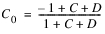


C and D are calculated as follows:


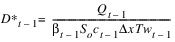
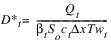
Q is the grid’s flow, So is the Energy Slope, c is the wave celerity, and Tw is the top width of the channel calculated for the given flow Q. The wave celerity c and Tw are found using the selected Depth to Flow method for the flow, Q, at the appropriate timestep (see Depth to Flow for details). The incremental timestep  is specified by the user while the spatial distribution
  is calculated to keep the Courant number close to 1 for the reference discharge.
is specified by the user while the spatial distribution is calculated to keep the Courant number close to 1 for the reference discharge. Method Details
The spatial distribution  is automatically calculated by RiverWare. The incremental spatial step is determined such that the Courant number, C, will be close to one to reduce the effects of numerical dispersion. Since the discharge will vary for a simulation, the Courant number will also vary. To pick a value for the incremental spatial step that minimizes the effects of numerical dispersion, the user inputs maximum and minimum discharges expected for a simulation in the Extreme Values slot. The average of these two discharges is used as the reference discharge. The wave celerity, c, is then computed with this reference discharge using the selected Depth to flow; see Depth to Flow for details. The spatial step size,
  is computed with the input
  and the Courant number, C set to be 1.0.
is automatically calculated by RiverWare. The incremental spatial step is determined such that the Courant number, C, will be close to one to reduce the effects of numerical dispersion. Since the discharge will vary for a simulation, the Courant number will also vary. To pick a value for the incremental spatial step that minimizes the effects of numerical dispersion, the user inputs maximum and minimum discharges expected for a simulation in the Extreme Values slot. The average of these two discharges is used as the reference discharge. The wave celerity, c, is then computed with this reference discharge using the selected Depth to flow; see Depth to Flow for details. The spatial step size, is computed with the input and the Courant number, C set to be 1.0.
The scheme is unconditionally stable for 0.0 <= X <= 0.5 or with D (cell Reynolds number) values less than unity. The cell Reynolds number, D, is defined as the ratio of hydraulic diffusivity to grid diffusivity, as follows:

where Q is the grid’s flow, So is the Energy Slope, c is the wave celerity, and Tw is the top width of the channel calculated for the given flow Q. Tw is found using the selected Depth to Flow method. X is related to D as follows:

The value of D for each numerical grid section for the current timestep can be observed in the Distributed MuskingumCunge Output table under the column labeled D.
Note: In this method if the flow result is very small or negative, C and D become 1, and X becomes 0.0. If the above equation for C0 results in a negative value, C and D are set to 1, and C0 is set to 0.
The value of C + D for each numerical grid section for the current timestep can be observed in the Distributed MuskingumCunge Output table under the column labeled C + D.
Method Steps
The method proceeds as follows.
1. Calculate the total inflow for the timestep (that is, the inflow plus local inflow minus diversion) to the reach.
2. The method loops through the incremental timesteps, t, and the spatial grid, i, to find the flow at each element  as follows.
as follows. a. FOR EACH incremental timestep, t
The inflow at each incremental timestep is determined by interpolating between the inflow for the previous day and the inflow for the current day. This is then set on the 0th column of the Distributed Flow Output slot
b. FOR EACH spatial step, i, in the grid
1. Estimate the flow  using the three point method.
using the three point method. 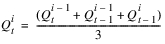
2. Using this flow, call the selected Depth to Flow method to determine ct, Twt, At.
3. Calculate  and
and  .
.
and . If the flow is zero, set  and
and  equal to 1.0.
and equal to 1.0.4. If the following does not hold true: 0.0 <=  <= 0.5, issue an error and stop the run. The scheme is not stable.
<= 0.5, issue an error and stop the run. The scheme is not stable. 5. Calculate C0, C1, and C2.


6. Calculate a new  using the Muskingum equation.
using the Muskingum equation.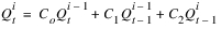
7. If the new  is within convergence of the old
  , go to the next spatial step, otherwise determine a new
  using a four point scheme, as follows:
is within convergence of the old , go to the next spatial step, otherwise determine a new using a four point scheme, as follows: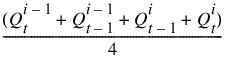
8. Return to step 2 and repeat until the flow,  , converges.
, converges.c. END FOR loop over spatial step, i
d. Compute Distributed Volume Output for each element in the reach as the previous incremental timestep’s Distributed Volume Output plus the average spatial flow in the reach.
e. END FOR loop over incremental timestep, t
3. Using the value in the last column of the Distributed Flow Output slot, execute the bankstorage and gain loss calculations, add in Return Flow, and execute negative outflow adjustment calculations. Each can add or subtract water from the reach. Set the resulting flow on the Outflow slot.
4. Finally, compute and set the Total Outflow Storage as the sum of the previous Total Outflow Storage plus the Outflow converted to a volume.
Note: To assure the routing parameters are appropriately computed for the given inflow, the reference flow along with corresponding values for the wave celerity and top width are used to compute new values for the cell Reynolds number, D, and the Courant number, C at each timestep. However, changing C and D values in the middle of a simulation results in a volume conservation error. Test results show that this error can be significant for sharply rising and falling hydrograph but the total volume conservation error over a flood event is less than 1%. See Muskingum-Cunge Improved for details on a similar method that better conserves mass.
This hydraulic routing method is an improvement to the Muskingum-Cunge method in which the coefficients are adjusted to better conserve mass as proposed by Todini, 20073.
Slots Specific to This Method
Delta X Computational Element Length
Type: 1X1 table slot
Units: Length
Description: size of the spatial discretization
Information: This slot is determined by the method, while it is input by the user for the other hydraulic routing methods.
I/O: Output only
Links: Not linkable
Distributed Celerity Output
Type: Table Series Slot
Units: Velocity
Description: celerity(wave speed) at each of the elements
Information: The value displayed in each row is the value for the last incremental timestep for each run timestep.
I/O: Output only; this is a temporary slot that is not saved in the model file.
Links: Not linkable
Distributed Courant Output
Type: Table Series Slot
Units: None
Description: The adjusted Courant value (C*) for each element in the reach.
Information: The value displayed in each row is the value for the last incremental timestep for each run timestep.
Note: In the iteration, the method uses the current and next timestep rows to store the previous and current values: current row = previous incremental timestep, next row = current incremental timestep. At the end of each incremental timestep, the value is copied from the next timestep’s row to the current timestep’s row. The only effect visible to the user of this iteration mechanism is that the last row of the table is the same as the last minus one row; the last row is beyond the end of the run and can be ignored.
I/O: Output only; this is a temporary slot that is not saved in the model file.
Links: Not linkable
Distributed Depth Output
Type: Table Series Slot
Units: Length
Description: depth of each element
Information: The value displayed in each row is the value for the last incremental timestep for each run timestep.
I/O: Output only; this is a temporary slot that is not saved in the model file.
Links: Not linkable
Distributed Flow Output
Type: Table Series Slot
Units: Flow
Description: Flow value of each element in the reach.
Information: The 0th column represents the flow to be routed (Inflow + Local Inflow - Diversion). The last column represents the routed flow; but the flow value displayed in each row is the flow in the last incremental timestep for each run timestep. This is not necessarily the same as the average over the run timestep. The Routed Flow slot holds this average over the incremental timesteps and is then used in subsequent calculations on the reach.
Note: In the iteration, the method uses the current and next timestep rows to store the previous and current values: current row = previous incremental timestep, next row = current incremental timestep. At the end of each incremental timestep, the value is copied from the next timestep’s row to the current timestep’s row. The only effect visible to the user of this iteration mechanism is that the last row of the table is the same as the last minus one row; the last row is beyond the end of the run and can be ignored.
I/O: Output only; this is a temporary slot that is not saved in the model file.
Links: Not linkable
Distributed MuskingumCunge Output
Type: Table
Units: Various
Description: holds output parameters of routing method.
Information: C0, C1, C2 are all reported here for the current timestep, along with D, C+D, X and K.
Note: C and D are also stored in the Distributed Courant Output and Distributed Reynolds Output slots.
I/O: Output only
Links: Not linkable
Distributed Previous Flow Output
Type: Table Series Slot
Units: Flow
Description: The Distributed Flow Output offset by one timestep
Information: This slot is used to store the previous distributed flow so that if the reach dispatch more than once, the distributed flow is not lost. The value displayed in each row is the value for the last incremental timestep for each run timestep.
I/O: Output only; this is a temporary slot that is not saved in the model file.
Links: Not linkable
Distributed Reynolds Output
Type: Table Series Slot
Units: None
Description: The adjusted Reynolds number (D*) for each element in the reach
Information: The value displayed in each row is the value for the last incremental timestep for each run timestep.
Note: In the iteration, the method uses the current and next timestep rows to store the previous and current values: current row = previous incremental timestep, next row = current incremental timestep.
At the end of each incremental timestep, the value is copied from the next timestep’s row to the current timestep’s row.
The only effect visible to the user of this iteration mechanism is that the last row of the table is the same as the last minus one row; the last row is beyond the end of the run and can be ignored.
I/O: Output only; this is a temporary slot that is not saved in the model file.
Links: Not linkable
Distributed TopWidth Output
Type: Table Series Slot
Units: Length
Description: width of top of water surface
Information: The value displayed in each row is the value for the last incremental timestep for each run timestep.
I/O: Output only; this is a temporary slot that is not saved in the model file.
Links: Not linkable
Distributed Velocity Output
Type: Table Series Slot
Units: Velocity
Description: velocity of each element
Information: The value displayed in each row is the value for the last incremental timestep for each run timestep.
I/O: Output only; this is a temporary slot that is not saved in the model file.
Links: Not linkable
Distributed Volume Output
Type: Table Series Slot
Units: Volume
Description: volume contained in each spatial element of the reach
Information: The value displayed in each row is the value for the last incremental timestep for each run timestep. This volume is the end of timestep value.
I/O: Output only; this is a temporary slot that is not saved in the model file.
Links: Not linkable
Distributed Xsectional Area Output
Type: Table Series Slot
Units: Area
Description: area of each element
Information: The value displayed in each row is the value for the last incremental timestep for each run timestep.
I/O: Output only; this is a temporary slot that is not saved in the model file.
Links: Not linkable
Energy Slope
Type: Scalar
Units: No Units
Description: slope of the reach from upstream to downstream (vertical/horizontal)
Information: Must be positive
I/O: Required input
Links: Not linkable
Extreme Flow Values
Type: 1X1 Table
Units: Flow
Description: base and max flow values expected during simulation run.
Information: Used for calculation of the routing distance step
I/O: Required input
Links: Not linkable
Max Iterations
Type: 1X1 Table Slot
Units: none
Description: This values specifies the maximum number of iterations used by convergence algorithm to compute the reach outflow.
I/O: Input; defaults to 20 if not set by the user
Links: Not linkable
Numerical Parameters Output
Type: Table
Units: Various
Description: Columns describing grid and Courant number of each element for the current timestep
Information: The rows of this table store the value of the Courant number with respect to distance. The number of rows used is based on the discretization parameters, Number of each Length/Delta X. The number of rows in this table is currently limited to 500.
I/O: Output only
Links: Not linkable
Previous Outflow
Type: Series Slot
Units: Flow
Description: Previous Outflow
Information: This is the outflow from the reach, offset by one timestep
I/O: Output only
Links: Linkable
Reach Length
Type: 1X1 Table Slot
Units: Length
Description: total length of the reach, from upstream to downstream.
Information:
I/O: Required input
Links: Not linkable
Reach Volume
Type: Series Slot
Units: Volume
Description: The volume of water in the reach at the end of the timestep.
Information: This volume is calculated as the sum of the Distributed Volume Output for each row. It is the sum of water over each spatial step along the reach.
I/O: Output only
Links: Not linkable
Return Flow
Type: Series Slot
Units: Flow
Description: return flow into the reach
Information: Enters at the bottom of the reach (that is, it is added directly to the Routed Flow calculated by the method).
I/O: Optional; if not input and not linked, it is set to zero.
Links: May be linked to the Return Flow slot on any object, the Outflow slot on a Groundwater Storage object, the Excess GW Outflow slot on the Groundwater Storage object, or the Surface Return Flow slot on a WaterUser.
Routed Flow
Type: Series Slot
Units: Flow
Description: The flow in the reach after routing has occurred but before gain/loss, return flow or bankstorage is added.
Information: This is calculated by averaging the downstream most distributed outflow from the reach over each of the incremental timesteps
I/O: Output only
Links: Not linkable
Routing Time Step
Type: 1X1 Table Slot
Units: Time
Description: timestep used by method,  in the equations below
in the equations belowInformation: This must be smaller than the simulation timestep. The value should be larger than the estimated time of travel for a wave through the reach. It must result in an exact integer number of routing timesteps per simulation timestep.
I/O: Required input
Links: Not linkable
Total Outflow Storage
Type: Series Slot
Units: Volume
Description: Cumulative volume of outflow throughout the run.
Information: It is calculated as the previous Total Outflow Storage plus the Outflow converted to a volume
I/O: Output only
Links: Not linkable
Background
The standard form of the Muskingum equation is as follows:
When applies to a spatially distributed grid, the flow in grid i is as follows:

where t is the incremental timestep at which the calculation is occurring. In the standard Muskingum-Cunge equation, C0, C1, and C2 are functions of the Courant number C and Reynolds number D.


C and D are calculated as follows:


Q is the grid’s flow, So is the Energy Slope, c is the wave celerity, and Tw is the top width of the channel calculated for the given flow Q. The wave celerity c and Tw are found using the selected Depth to Flow method for the flow, Q, at the appropriate timestep (see Depth to Flow). The incremental timestep  is specified by the user while the spatial distribution
  is calculated to keep the Courant number close to 1 for the reference discharge.
is specified by the user while the spatial distribution is calculated to keep the Courant number close to 1 for the reference discharge.In the variable parameter, Muskingum-Cunge routing method, the cell Reynolds number, D, and the Courant number, C change at each timestep for each cell. Changing C and D values in the middle of a simulation results in a volume conservation error and storage inconsistency at steady state as shown by Todini. See Muskingum-Cunge for details.
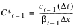
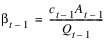
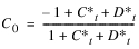
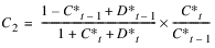
To mitigate this loss of mass, Todini rederived the equations (not shown) and calculated the coefficients as follows:


Where C* and D* are the corrected Courant number and Reynolds number, respectively, as follows:


The Muskingum-Cunge Improved method is an implementation of this scheme. Although Todini proposed relationships to define the channel parameters for common channel geometry, this method uses an iterative 3 and 4 point scheme and the selected Depth to Flow method to determine these same parameters (area, top width, depth, velocity, and celerity).
In addition, the reach inflow is used as the inflow to each incremental timestep. The Outflow is an average of the outflow over each incremental timestep. Full details of this method follow the slot descriptions.
Method Details
The incremental timestep  is related to the spatial distribution
  as follows:
is related to the spatial distribution as follows:
Since the discharge varies for a simulation, the Courant number will also vary. To pick a value for the incremental spatial step that minimizes the effects of numerical dispersion, the user inputs minimum and maximum discharges expected for a simulation in the Extreme Flow Values slot. The average of these two discharges is used as the reference discharge when computing the wave celerity, c, using the selected Depth to Flow method. Then, the incremental spatial step  is determined with the Courant number, C, set equal to 1.0 to reduce the effects of numerical dispersion.
is determined with the Courant number, C, set equal to 1.0 to reduce the effects of numerical dispersion. 
Note: This routing method loops over the incremental timestep, which must be smaller than the run timestep. The values displayed in the Distributed Output slots are the values for the last incremental timestep. The incremental values are strictly internal and there is no way to show the values for intermediate incremental timesteps.
Method Steps
The method proceeds as follows.
1. Calculate the inflow (that is, the inflow plus local inflow minus diversion) to the reach and set the flow in the 0th column of the Distributed Flow Output slot equal to this flow. This same inflow value is used for each incremental timestep (no interpolation is used as in the original, as this leads to a further mass inconsistency; see Muskingum-Cunge). Using this inflow, call the selected Depth to Flow method to determine c, Tw, and At. Calculate  and
and  using those values. Set the 0th column of the appropriate table series slot.
and using those values. Set the 0th column of the appropriate table series slot.2. The method loops through the incremental timesteps, t, and the spatial grid, i, to find the flow at each element  as follows.
as follows. 3. FOR EACH incremental timestep, t
a. FOR EACH spatial step, i, in the grid
1. Estimate the flow  using the three point method.
using the three point method. 2. Using this flow, call the selected Depth to Flow method to determine ct, Twt, At.
3. Calculate 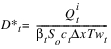 and
and  where
where  .
.
and where . If the flow is zero, set  and
and  equal to 1.0.
and equal to 1.0.4. If the following does not hold true: 0.0 <=  <= 0.5, issue an error and stop the run. The scheme is not stable.
<= 0.5, issue an error and stop the run. The scheme is not stable. 5. Calculate C0, C1, and C2.

Note:  and
and  are from the previous incremental timestep and were stored in the appropriate cell of the respective table series slot.
and are from the previous incremental timestep and were stored in the appropriate cell of the respective table series slot.6. Calculate a new  using the Muskingum equation.
using the Muskingum equation. 
7. If the new  is within convergence of the old
  , go to the next spatial step, otherwise determine a new
  using a four point scheme.
is within convergence of the old , go to the next spatial step, otherwise determine a new using a four point scheme.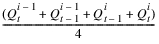
8. Return to step 2 and repeat until the flow,  , converges. Once convergence occurs, set a temporary variable tempOutflowVolume to track the total volume of outflow (last column of the Distributed Flow Output slot; that is, the bottom of the reach). Add to this total volume at each incremental timestep.
, converges. Once convergence occurs, set a temporary variable tempOutflowVolume to track the total volume of outflow (last column of the Distributed Flow Output slot; that is, the bottom of the reach). Add to this total volume at each incremental timestep.b. END FOR loop over spatial step, i
c. Compute Distributed Volume Output for each element in the reach, as follows:
4. END FOR loop over incremental timestep, t.
5. Next, the Routed Flow is calculated as the average outflow over the incremental timesteps. This is calculated by dividing the tempOutflowVolume by the run timestep. Then, sum up the Distributed Volume Output over space (that is, a given row) and set this value on the Reach Volume slot.
6. Using the Routed Flow, execute the bankstorage and gain loss calculations, add in Return Flow, and execute negative outflow adjustment calculations. Each can add or subtract water from the reach. Set the resulting flow on the Outflow slot.
7. Finally, compute and set the Total Outflow Storage as the sum of the previous Total Outflow Storage plus the Outflow converted to a volume.
This method was implemented to achieve better mass conservation but is not guaranteed to fully conserve mass. Because the user selects the Extreme Flow values and Routing Timestep, there are circumstances where flow is not fully conserved. This is especially true when there are abrupt flow changes and flows that are zero. Testing has shown that mass is fully conserved in well behaved problems but not necessarily in real-world problems. Regardless, the mass conservation is much better than the original routing method.
This hydraulic routing method is a finite difference solution of the kinematic wave simplification to the St. Venant Equations. It requires a numerical grid to be specified by the user.
Slots Specific to This Method
Delta X Computational Element Length
Type: Scalar
Units: LENGTH
Description: size of the x discretization
Information: This slot must be smaller than the Reach Length.
I/O: Required input
Links: Not linkable
Distributed Celerity Output
Type: Table Series
Units: VELOCITY
Description: celerity(wave speed) at upstream end of each elements
Information: This is a temporary slot that is not saved in the model file.
I/O: Output only
Links: Not linkable
Distributed Depth Output
Type: Table Series
Units: LENGTH
Description: depth at upstream end of each element
Information: This is a temporary slot that is not saved in the model file.
I/O: Output only
Links: Not linkable
Distributed Flow Output
Type: Table Series
Units: FLOW
Description: inflow value at the upstream end of each element
Information: This is a temporary slot that is not saved in the model file.
I/O: Output only
Links: Not linkable
Distributed TopWidth Output
Type: Table Series
Units: LENGTH
Description: width of top of water surface
Information: This is a temporary slot that is not saved in the model file.
I/O: Output only
Links: Not linkable
Distributed Velocity Output
Type: Table Series
Units: VELOCITY
Description: velocity at upstream end of each element
Information: This is a temporary slot that is not saved in the model file.
I/O: Output only
Links: Not linkable
Distributed Volume Output
Type: Table Series
Units: VOLUME
Description: volume contained in each element
Information: This is a temporary slot that is not saved in the model file.
I/O: Output only
Links: Not linkable
Distributed Xsectional Area Output
Type: Table Series
Units: AREA
Description: area at upstream end of each element
Information: This is a temporary slot that is not saved in the model file.
I/O: Output only
Links: Not linkable
Numerical Parameters Output
Type: Table
Units: VARIOUS
Description: Columns describing grid and Courant number of each element for the current timestep
Information: The rows of this table store the value of the Courant number with respect to distance. The number of rows used is based on the discretization parameters defined by the user, Number of each Length/Delta X. The number of rows in this table is currently limited to 500; therefore, the number of computational elements for each reach must not be greater than 500; that is, Delta X must not be less than Reach Length/500.
I/O: Output only
Links: Not linkable
Reach Length
Type: Scalar
Units: LENGTH
Description: total length of the reach, from upstream to downstream.
Information: This slot must be larger than Delta X
I/O: Required input
Links: Not linkable
Return Flow
Type: Series
Units: FLOW
Description: return flow into the reach
Information: Enters at the bottom of the reach (that is, added directly to the outflow calculated by the method).
I/O: Optional; if not input and not linked, it is set to zero.
Links: May be linked to the Return Flow slot on any object, the Outflow slot on a Groundwater Storage object, the Excess GW Outflow slot on the Groundwater Storage object, or the Surface Return Flow slot on a WaterUser.
Routing Time Step
Type: Table
Units: TIME
Description: timestep used by method
Information: This must be smaller than the simulation timestep. The value should be larger than the estimated time of travel for a wave through the reach.
I/O: Required input
Links: Not linkable
Method Details
The solution is a nonlinear numerical approximation to the following continuity and momentum equations.
Continuity 
Momentum 
For this numerical solution, accuracy increases as the Courant number approaches unity and decreases as the Courant number diverges from unity. The Courant number for each numerical grid section for the current timestep can be observed in the Numerical Parameters Output under the column labeled Courant. The Courant number is calculated as follows:

where c = wave celerity [L/T],  t = routing time step[T], and
  x = spatial step size[L].
t = routing time step[T], and x = spatial step size[L].This hydraulic routing method also requires the user to select from another category of user selectable methods: Depth to Flow. The inputs for these methods are described under that user method category.
The algorithm uses is a predictor corrector scheme that is unstable for a Courant number greater than unity. The advantage of this scheme is that it is second order accurate and can minimize numerical diffusion. The general equations for this method are as follows.
Predictor 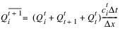
Corrector 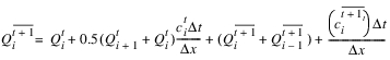
This method is a simple storage method that solves for outflows given current and previous inflow values. The reach is broken up into a user-specified number of linked segments and flows are calculated for each segment.
Note: This method is based on an empirical formula that uses a numeric approximation; therefore the method does not guarantee that mass balance will be preserved exactly.
Slots Specific to This Method
Number of Segments in Reach
Type: Scalar
Units: NOUNITS
Description: number of segments upstream to downstream
Information: This will determine the number of columns in the Segment Outflow table as well.
I/O: Required input
Links: Not linkable
Segment Outflow
Type: Table Series
Units: FLOW
Description: segment outflow
Information: The outflow from the reach is the outflow from the last segment. The columns in this table will be resized to the number of segments input by the user, and the number of rows will be the number of timesteps in the run.
I/O: Output only; this is a temporary slot that is not saved in the model file.
Links: Not linkable
Storage Time Coefficient
Type: Scalar
Units: NOUNITS
Description: value that is divided by the result of the average flow and exponent to arrive at time in storage
Information: The units of this slot should be Volumeexponent (a value should be used that is in (ft3)exponent). This coefficient may be determined by trial and error, and should not be negative. The value must correspond to a flow value in cfs and storage time in hours, regardless of the user units on other slots.
I/O: Required input
Links: Not linkable
Storage Time Exponent
Type: Scalar
Units: NOUNITS
Description: exponent of mean flow value.
Information: Usually between -1 and 1. The value must correspond to a flow value in cfs and storage time in hours, regardless of the user units on other slots.
I/O: Required input
Links: Not linkable
Method Details
The algorithm proceeds as follows.
1. If the previous Inflow value is not known, the method exits.
2. The outflow value for each segment from the previous timestep is checked for validity. There are then three possible scenarios:
– If the segment outflows are not valid and previous Outflow is not valid, Outflow is set equal to inflow plus gain loss and the method exits.
– If the segment outflows are not valid, and previous Outflow is valid, set all segment outflows equal to previous Inflow, and continue the routing method.
– If the segment outflows are valid, continue the method.
3. Find the mean interior flow from the previous timestep as the average of all segment outflows.
4. Find the time of storage in the reach based on the following empirical formula(in cfs).
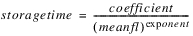
where storagetime is the time of storage in hours; coefficient and exponent are user input constants in the slots above; and meanfl is the average interior flow of the previous timestep.
Note: The storagetime calculation is always made with meanfl in units of cfs regardless of the user units on any flow slots. The values for Storage Time Coefficient and Storage Time Exponent should be set accordingly.
The time in storage can be used as a conversion from storage to outflow.

5. Find the number of routing phases, n. If the time of storage is greater than half of the simulation timestep, n is 1. Otherwise, n is calculated as follows:
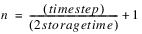
If n is greater than 48 from this equation, n is set to 6.
6. The inflow into the first segment for each routing phase is calculated as follows:
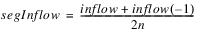
7. For each routing phase, the outflow from each segment is calculated as follows:

This routing equation is based on the storage-outflow relation, storagetime, from above, and the continuity equation.

8. The inflow into the next segment is the average of the segments previous and current outflows
9. The current timestep’s Outflow for the object is equal to the last segment’s outflow.
This method is a simple storage method that solves for outflows given current and previous inflow values. The reach is broken up into a user-specified number of linked segments and flows are calculated for each segment. This method differs from the Storage Routing method only in the determination of the storagetime value. In this method, the storage time exponent and coefficient are found from a table lookup based on flow instead of constant values.
Note: This method is based on an empirical formula that uses a numeric approximation; therefore the method does not guarantee that mass balance will be preserved exactly.
Slots Specific to This Method
Flow Range
Type: Table
Units: FLOW
Description: the ranges of flow rates corresponding to the Variable Storage Time Tables
Information: The number of flow ranges allowed in this table is currently limited to 10. The columns of this table represent, in ascending order, the maximum flow rate for a specific flow range starting with 0 as the base. These columns are labeled Flow Range 1 - 10. Therefore, the first column represents a range of flows from 0 to the value input by the user in the Flow Range 1 column. The last flow range entered by the user should be a flow rate greater than any anticipated for the simulation. Otherwise, a value of 0.0 will be used for the Variable Storage Time slots for flows outside of this range. It is not necessary to utilize all 10 columns of this table. Use only the columns needed to designate the desired flow ranges.
I/O: Required input
Links: Not linkable
Number of Segments in Reach
Type: Scalar
Units: NOUNITS
Description: number of segments upstream to downstream
Information: This will determine the number of columns in the Segment Outflow table as well.
I/O: Required input
Links: Not linkable
Segment Outflow
Type: Table Series
Units: FLOW
Description: segment outflow
Information: The outflow from the reach is the outflow from the last segment. The columns in this table will be resized to the number of segments input by the user, and the number of rows will be the number of timesteps in the run.
I/O: Output only; this is a temporary slot that is not saved in the model file.
Links: Not linkable
Variable Storage Time Coefficient
Type: Series
Units: NOUNITS
Description: value that is divided by the result of the average flow and exponent to arrive at time in storage
Information: The units of this slot should be Volumeexponent (a value should be used that is in (ft3)exponent).
I/O: Output only
Links: Not linkable
Variable Storage Time Coefficient Table
Type: Table
Units: NOUNITS
Description: Variable Storage Time Coefficient for each specific Flow Range
Information: The columns of the table correspond to the flow ranges defined in Flow Range. The values must correspond to a flow value in cfs and storage time in hours, regardless of the user units on other slots.
I/O: Required input
Links: Not linkable
Variable Storage Time Exponent
Type: Series
Units: NOUNITS
Description: exponent of mean flow value.
Information: Usually between -1 and 1.
I/O: Output only
Links: Not linkable
Variable Storage Time Exponent Table
Type: Table
Units: NOUNITS
Description: Variable Storage Time Exponent for each specific Flow Range
Information: The columns of the table correspond to the flow ranges defined in Flow Range. The values must correspond to a flow value in cfs and storage time in hours, regardless of the user units on other slots.
I/O: Required input
Links: Not linkable
Method Details
The algorithm proceeds as follows.
1. If the previous Inflow value is not known, the method exits.
2. The outflow value for each segment from the previous timestep is checked for validity. There are then three possible scenarios:
– If the segment outflows are not valid and previous Outflow is not valid, Outflow is set equal to inflow plus gain loss and the method exits.
– If the segment outflows are not valid, and previous Outflow is valid, set all segment outflows equal to previous Inflow, and continue the routing method.
– If the segment outflows are valid, continue the method.
3. Find the mean interior flow from the previous timestep as the average of all segment outflows.
4. Find the time of storage in the reach based on the following empirical formula(in cfs).

where storagetime is the time of storage in hours; coefficient and exponent are user input constants in the slots above; and meanfl is the average interior flow of the previous timestep.
Note: The storagetime calculation is always made with meanfl in units of cfs regardless of the user units on any flow slots. The values in the Variable Storage Time Coefficient Table and Variable Storage Time Exponent Table should be set accordingly.
The time in storage can be used as a conversion from storage to outflow.

5. Find the number of routing phases, n. If the time of storage is greater than half of the simulation timestep, n is 1. Otherwise, n is calculated as follows:
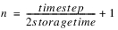
If n is greater than 48 from this equation, n is set to 6.
6. The inflow into the first segment for each routing phase is calculated as follows:

7. For each routing phase, the outflow from each segment is calculated as follows:
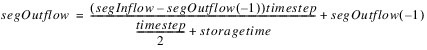
This routing equation is based on the storage-outflow relation, storagetime, from above, and the continuity equation, as follows:

8. The inflow into the next segment is the average of the segments previous and current outflows
9. The current timestep’s Outflow for the object is equal to the last segment’s outflow.
The Modified Puls algorithm solves for the Reach Outflow given current and previous Inflow and Storage values using the following continuity equation, as follows:

Rewritten, this equation is as follows:

The equation has two unknowns, Storage and Outflow, both on the left side. In the Modified Puls method, the user specifies a tabular relationship of Storage versus Outflow in the Storage Outflow Table. Given this table of data, the set of Storage and Outflow can be found to satisfy the equation.
You can further discretize the reach into n sub-reaches for better control over the attenuation of the flood wave. The Storage Outflow Table is specified for the entire reach. Therefore, during the solution, the Storage in each subreach is assumed to be 1/n of the total storage. Each subreach is assumed to be identical and uniform.
This routing method is called from the Solve given Inflow, Storage Routing dispatch method. That is, when Modified Puls is selected, the only available dispatch method is Solve given Inflow, Storage Routing. This dispatch method solves downstream and includes optional Bank Storage, Gain Loss, Outflow Adjust, Stage, and Volume calculations.
Note: All these calculations occur after the routing has occurred, based on the routed flow.
Slots Specific to This Method
Number of Segments in Reach
Type: Scalar
Units: None
Description: Number of segments
Information: This parameter determines the number of columns in the Segment Outflow table. The travel time through a segment should be approximately equal to the timestep size. An estimate is to divide the reach length by the product of the wave celerity and timestep size. In the equations below, the number of segments is represented by the variable n.
I/O: Required input
Links: Not linkable
Outflow by Segment
Type: Agg Series
Units: FLOW
Description: Segment outflow. The segments are numbered upstream to downstream. The Outflow to one segment is the inflow to the next segment.
Information: The outflow from the reach is the outflow from the last segment. The columns in this slot will be resized to the number of segments input by the user, and the number of rows will be the number of timesteps in the run. At the beginning of the run, if the initial timestep Outflow by Segment is not known, the Outflow by Segment is set to the Reach Inflow or Outflow, if known.
Information: Input at Initial timestep, Output at other timesteps
I/O: Output only
Links: Not linkable
Storage by Segment
Type: Agg Series
Units: Volume
Description: Segment storage. The segments are numbered upstream to downstream, left to right.
Information: The columns in this table will be resized to the number of segments input by the user, and the number of rows will be the number of timesteps in the run.
I/O: Output only
Links: Not linkable
Storage Outflow Table
Type: Table
Units: Volume vs Flow
Description: The table relating Storage in the entire reach to the Outflow.
Information: The data must be monotonically increasing and cover the entire range of storage and flow values expected.
I/O: Input only
Links: Not linkable
Storage Outflow Indication Table
Type: Table
Units: Volume vs Flow vs Flow
Description: This generated table repeats the Storage Outflow Table and then shows a third column for the Indication variable.
Information: This table is generated at the beginning of run by looking up each Storage and Outflow on the Storage Outflow Table. These become the first and second columns. The third column, the Indication, is computed by looking up each row’s Storage and Outflow and then computing the value.
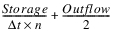
Information: Thus, the Indication is for a single segment. All segments are assumed to be the same. In addition, the timestep length is assumed to be constant.
I/O: Output only. This table is read only.
Links: Not linkable
Method Details
First, the method checks the following.
1. The current timestep’s inflow is checked. It should be known or the dispatch method would not have been called.
2. If the previous Inflow is not known, the method exits and waits.
3. The Outflow by Segment from the previous timestep is checked for validity. If they are all valid from previous solutions, they are used directly and the method continues. If any of the Outflow by Segment are not valid, the following checks are made:
a. If the Outflow is not known and the last Outflow by Segment is known, then Outflow is set to that value. All other Outflow by Segments are also set to that value.
b. Else, if the Outflow is not known, Outflow and each Outflow by Segment is set equal to the Inflow and the routing method exits. This scenario can occur the first time the reach dispatches. This situation is used when you would like the initial Outflow = Inflow.
c. If the Outflow is known (input or set by a rule), each Outflow by Segment is set equal to the Outflow and the method exits. This scenario can occur the first time the reach dispatches and achieves the need where initial Outflow is specified.
4. If the previous Storage values for each segment are not known, the method computes the previous Storage from the Storage Outflow Table.
5. Next, the method sets up arrays of the variables I, S, and O with the known information. The arrays will have 2 rows (timesteps) and n columns (segments).
Note: I(t, 1) = Inflow. Table 23.2 shows the array with the variables. Those next to each other are set to the same value, for example O(t-1,2) = I(t-1,3).
Timestep | Reach | Segment 1 | Segment 2 | Segment3 | Reach | ||||||
|---|---|---|---|---|---|---|---|---|---|---|---|
t-1 | Inflow(t-1) | I(t-1,1) | S(t-1,1) | O(t-1,1) | I(t-1,2) | S(t-1,2) | O(t-1,2) | I(t-1,3) | S(t-1,3) | O(t-1,3) | Outflow(t-1) |
t | Inflow(t) | I(t,1) | S(t,1) | O(t,1) | I(t,2) | S(t,2) | O(t,2) | I(t,3) | S(t,3) | O(t,3) | Outflow(t) |
6. Next, loop over each segment and compute the outflow and storage for each segment upstream to downstream:
For (j=1 to Number of Segments)
Compute the StorOutIndication variable.
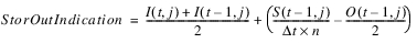
If StorOutIndication is less than zero, reset it to zero.
Look up the StorOutIndication on the Storage Outflow Indication Table to find the Storage and Outflow.
Record the values found as S(t,j) and O(t,j).
Set the inflow value for the next segment, I(t,j+1) = O(t,j)
End For
7. Set the slots Storage by Segment[t,j], Outflow by Segment[t,j] to the values stored in the arrays.
8. Execute Reach Bank Storage and Reach GainLoss method using the routed flow (Outflow in the last segment)
9. Set the Reach Outflow equal to the last segment’s outflow plus Bank Storage Return flow plus Total Gain Loss.
10. Execute the selected Outflow Adjustment method and reset Outflow if necessary
11. Return to the Solve given Inflow, Storage Routing dispatch method.
1 Chow, Ven Te, David R. Maidment, and Larry W. Mays. Applied Hydrology. McGraw-Hill, NewYork, 1988.
2 Chow, Ven Te, David R. Maidment, and Larry W. Mays. Applied Hydrology. McGraw-Hill, NewYork, 1988.
3 Todini, E. 2007, A mass conservation and water storage consistent variable parameter Muskingum-Cunge approach, Hydrology and Earth System Sciences, vol 11, 1645-1659) http://www.hydrol-earth-syst-sci.net/11/1645/2007/hess-11-1645-2007.pdf
Revised: 08/02/2021