
Simulation Diagnostics
Figure 3.7 is a sample Simulation Diagnostic Configuration Dialog. Available filters include Object, Timestep, and Slots.
Figure 3.7
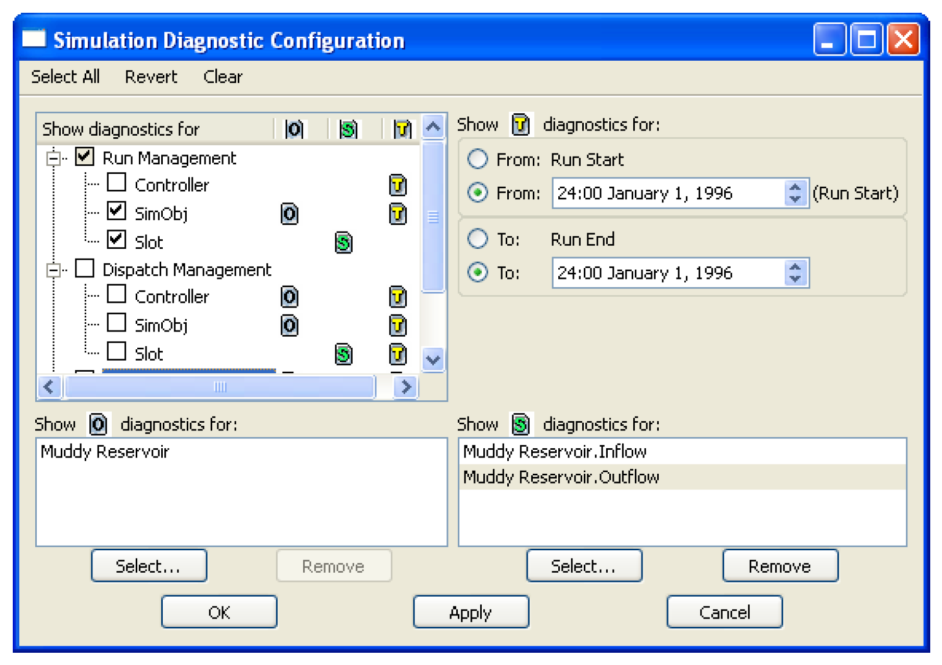
Table 3.2 summarizes the types of messages that are displayed when a Diagnostic Group is selected.
Super Group | Diagnostics Group | Type of diagnostics issued |
|---|---|---|
Run Management: | ||
Controller | Beginning/End of Run/Timestep for each time. Examples: • Initializing model run. • Beginning of Run. • Begin Timestep. • Execute timestep. • End of run. | |
SimObj | Beginning/End of Run/Timestep for each Object and time. Examples: • Clear state. • Propagating user input. • Beginning of run. • Begin timestep. • End timestep. • End of run. | |
Slot | Beginning of Run for each Slot and time. Examples: • Clear state. • Propagating user input. | |
Dispatch Management: | ||
Controller | Beginning of a dispatch for each object and time. Example: • Executing dispatch method (Solve given Inflow, Outflow) at Priority 7. | |
SimObj | Dispatch readiness for each object and time. Examples: • Slot (“Inflow”) added to known set. • Ready for dispatch method (“Solve given Inflow, No Routing”). • Slot (“Inflow”) is already in known set. • Re-dispatching using slot priorities. Priority 3R:Inflow Priority 7:Outflow Priority 7:Total Diversion Priority 7:Total Return Flow Priority 7:Total Local Inflow Conflicting slot values:(“Inflow” “Outflow” “Total Diversion” “Total Return Flow” “Total Local Inflow”). | |
Slot | Value assignments and propagation for each slot and time. Examples: • Set value = 453.003351 *1000.0 acre-feet/month = 208.621343 *1.0cms. • Propagate value to slot (“Total Available Water”). | |
Independent Groups: | ||
User Methods | Execution of User Methods for each object and time. Example: • Executing the user method “Daily Evaporation” in the category “Evaporation and Precipitation”. | |
Interpolation | TableSlot table interpolation lookups for each slot. Examples: • Table Interpolation 2 (3D) Specified z value (960.6579) falls between row ranges (556-572) and (573-589). (1->2) rows (556-572) x=195.804788, y=198.503173 (1->2) rows (573-589) x=195.804788, y=198.585469 (fixed 0 at 960.657920, 1->2) (in=195.804788) (out=198.579323 slope=.656000 intercept=70.131382) | |
Client Server | Provides information on the Client Server interaction. This includes the RiverWare - DSS, RiverWare - HDB, and RiverWare - MODFLOW connections. | |
Expr. Slot Execution | Expression slot execution are printed for expression slots that are configured to evaluate during a run (evaluation time of beginning or end of timestep or beginning or end of run). Example: • Expression evaluated to 624.00 [1000 acre-ft] | |
Expr. Slot Function Execution | Evaluation of RPL functions called by expression slots evaluated during a run. Diagnostics messages are printed for function execution (both user defined and predefined). “Before Execution” function diagnostics show the function being called and the arguments passed into the function. “After Execution” function diagnostics show the value that the function evaluated to and whether or not the value was constrained. Note: Function diagnostics also need to be enabled on the functions themselves. This can be done through the Function Editor dialog (for enabling diagnostics on individual functions) or by selecting Set, then Function Diagnostics from the main Set Editor (for enabling or disabling function diagnostics for all functions in the set). The Expression Slot Set editor is accessed from the Workspace Policy, then Open Expression Slot RPL Set. See Function Diagnostics for details on configuring the diagnostics. See Series Slots With Expression in User Interface for details on expression slots. Example: • SumFlowsToVolume($”Mountain Storage.Inflow”, @”Start Timestep”, @”t”) • “SumFlowsToVolume” evaluated to: 274839.74 [“m3”]. | |
Init. Rules Rule Execution | Initialization Rules rule execution diagnostics are printed for each rule. For a Simulation run, there is no filtering based on rule name. When enabled, diagnostics are shown for all Initialization rules. Examples: • Executing rule (#3) Assignment initiated (the left-hand side is “Mohave.Storage”[]) Evaluation of Assignment statement successful; will attempt assignment Mohave.Storage[July, 1998] = 1590800.00 [1.00 acre-ft] Rule successfully finished • Early termination: NaN encountered. The problem was encountered at the following location within the expression: “FC Violation”(). • RHS of assignment evaluated to NaN. | |
Init. Rules Function Execution | Diagnostics messages for function execution (both user defined and predefined) from initialization rules. For a Simulation run, there is no filtering based on rule name. When enabled, diagnostics are shown for all Initialization rules. “Before Execution” function diagnostics show the function being called and the arguments passed into the function. “After Execution” function diagnostics show the value that the function evaluated to and whether or not the value was constrained. Note: Function diagnostics also need to be enabled on the functions themselves. This can be done through the Function Editor dialog (for enabling diagnostics on individual functions) or by selecting Ruleset, then Ruleset Function Diagnostics from the main Ruleset Editor (for enabling or disabling function diagnostics for all functions in the ruleset). See Function Diagnostics for details. Examples: • GetMaxReleaseGivenInflow (% “WattsBar”, 0.634 [“1000 * cms”], @”Current Timestep”) • “GetMaxReleaseGivenInflow” evaluated to: 1299.413 [“cms”] • “GetMaxReleaseGivenInflow” constrained to: 1200.00 [“cms”] | |
Init. Rules Print Statements | User defined messages for each initialization rule. For a Simulation run, there is no filtering based on rule name. When enabled, diagnostics are shown for all Initialization rules. Example: • Entering rule curve routine for January - July | |
Revised: 01/04/2021