
Objects and Methods
Table Interpolation
This section describes the RiverWare algorithms for approximating continuous functions using linear interpolation between a sample of points defining the function. This data is input by the user into data tables (Table Slots); thus we refer to this approach to function approximation as table interpolation.
About Table Interpolation
Table interpolation occurs in the following contexts:
• Execution of some user methods during simulation. For example, the Plant Efficiency Curve method in the Power Calculation category on power reservoirs performs a three-dimensional table interpolation on the Plant Power Table.
• An optimization run, as part of the process of approximating nonlinear functions as one or more linear functions. For example, linearizing which used the Stage Flow Tailwater Table on power reservoirs.
• A rules or accounting run in which a RPL block executes the interpolation function. For example, the user could create a table on a data object representing evaporation as a function of temperature. Within a rule one could use two-dimensional interpolation to find the evaporation corresponding to any temperature in the range of this table.
RiverWare supports table interpolation for functions of two and three dimensions.
• For functions of two variables, it is useful to refer to the table columns as x and y, where x is the independent variable and y is the dependent variable: y = f(x).
• For functions of three variables, we refer to the columns as x, y, and z, where y = f(x, z).
We denote a particular approximation using the table by an asterisk: y* = f(x*) or y* = f(x*, z*)
Two-dimensional Data Format
For two-dimensional interpolation, RiverWare assumes that the values in the x column of the data table are increasing. Table B.1 is an example of the proper way to formulate a table for two-dimensional interpolation.
Pool Elevation (ft) | Storage (acre-ft) |
|---|---|
440 | 439,400 |
441 | 455,900 |
442 | 472,600 |
443 | 489,600 |
445 | 507,000 |
Two-dimensional Table Interpolation
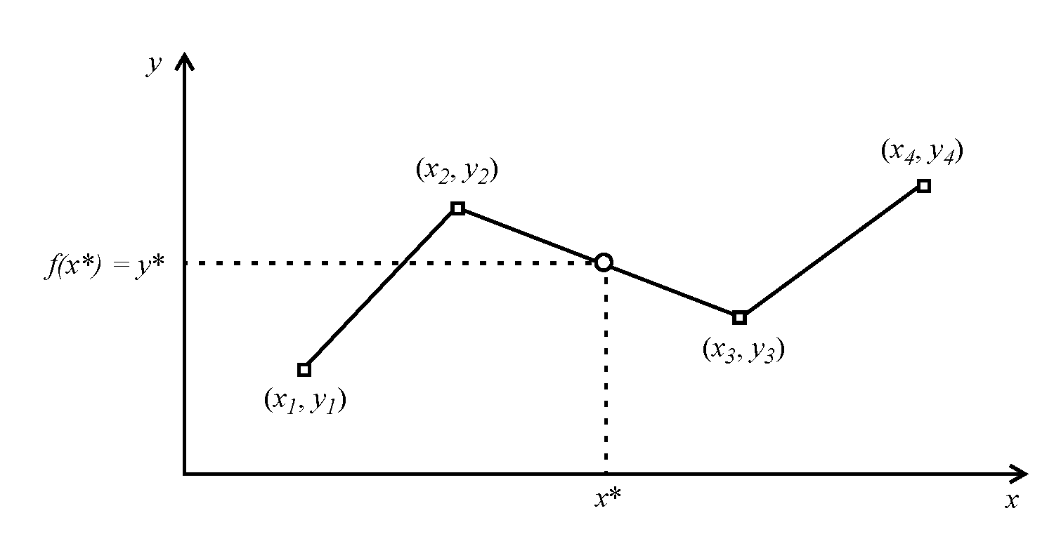
For two-dimensional functions, we apply linear interpolation between data points. Figure B.1 illustrates this approach.
Figure B.1 Two-dimensional linear interpolation
Two-dimensional Table Interpolation Errors
The following types of errors may be reported during two-dimensional table interpolation:
• Invalid value (data error): an x or y value is invalid (xi = NaN or yi = NaN, for some i).
• Non-increasing x (data error): the x values are not increasing (xi >= xi-1, for some i).
• Out of range (interpolation error): the x value being interpolated is out of the range of the table, that is, the domain of the function being approximated (x* < xmin or x* > xmax).
Three-dimensional Data Format
For three-dimensional interpolation, the z values define blocks: each block has a constant z value and increasing x values, and the blocks are arranged in order of increasing z value. In other words, the three-dimensional surface is represented by multiple slices or contours in the x-y plane, each of which may be represented by any arbitrary number of data points, just as with ordinary two-dimensional curves. Table B.2 is an example of the proper way to formulate a table for three-dimensional interpolation.
Operating Head (ft) | Turbine Release (cfs) | Power (kW) |
|---|---|---|
100 | 0 | 0 |
100 | 10 | 2000 |
100 | 20 | 3000 |
100 | 30 | 4000 |
200 | 0 | 0 |
200 | 10 | 2500 |
200 | 20 | 3500 |
200 | 25 | 3800 |
200 | 30 | 4500 |
300 | 0 | 0 |
300 | 10 | 3000 |
300 | 25 | 5000 |
Three-dimensional Table Interpolation
For three-dimensional functions, the algorithm for interpolation has two basic cases, as follows:
• If the z value being interpolated is equal to the z value for one of the blocks in the table, then we just perform a two-dimensional interpolation along the curve represented by that block.
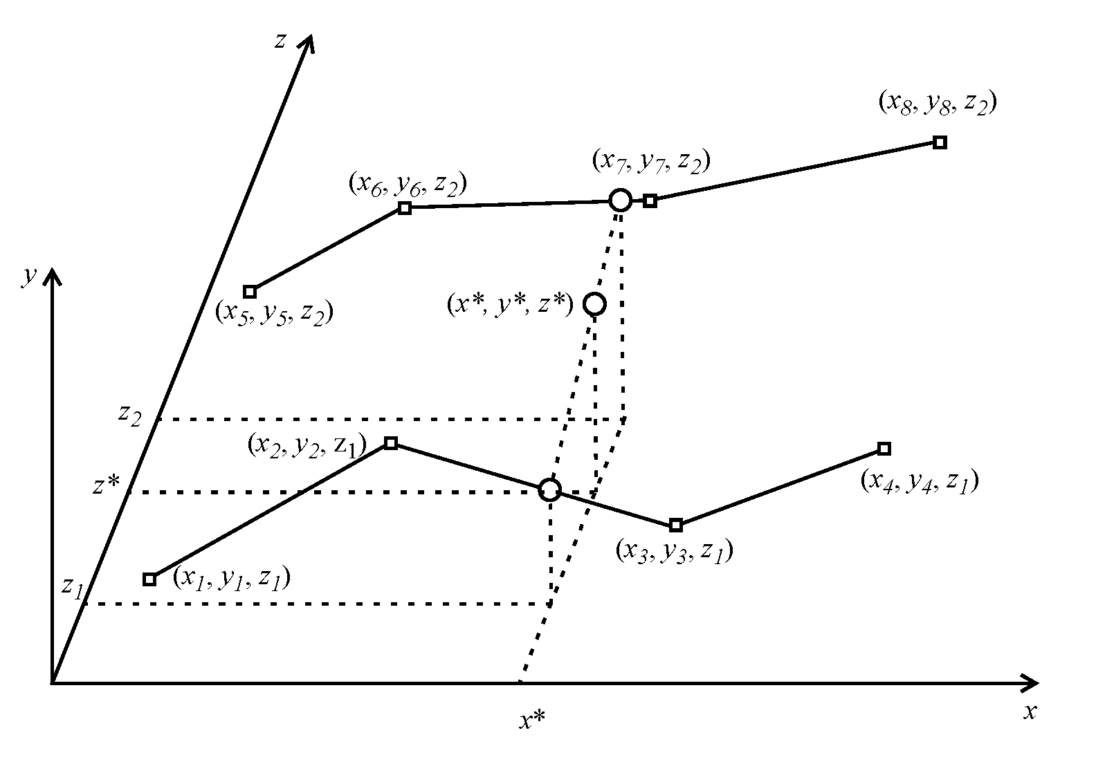
• When the z value is not exactly equal to any of the z values found in the table, RiverWare first identifies the constant z-blocks whose values bound the z value being interpolated and performs a two-dimensional interpolation along these curves. This yields two points, one on each bounding constant z-curve, and the final answer is computed by a linear interpolation between these two points. Figure B.2 illustrates this case.
Figure B.2 Three-dimensional linear interpolation
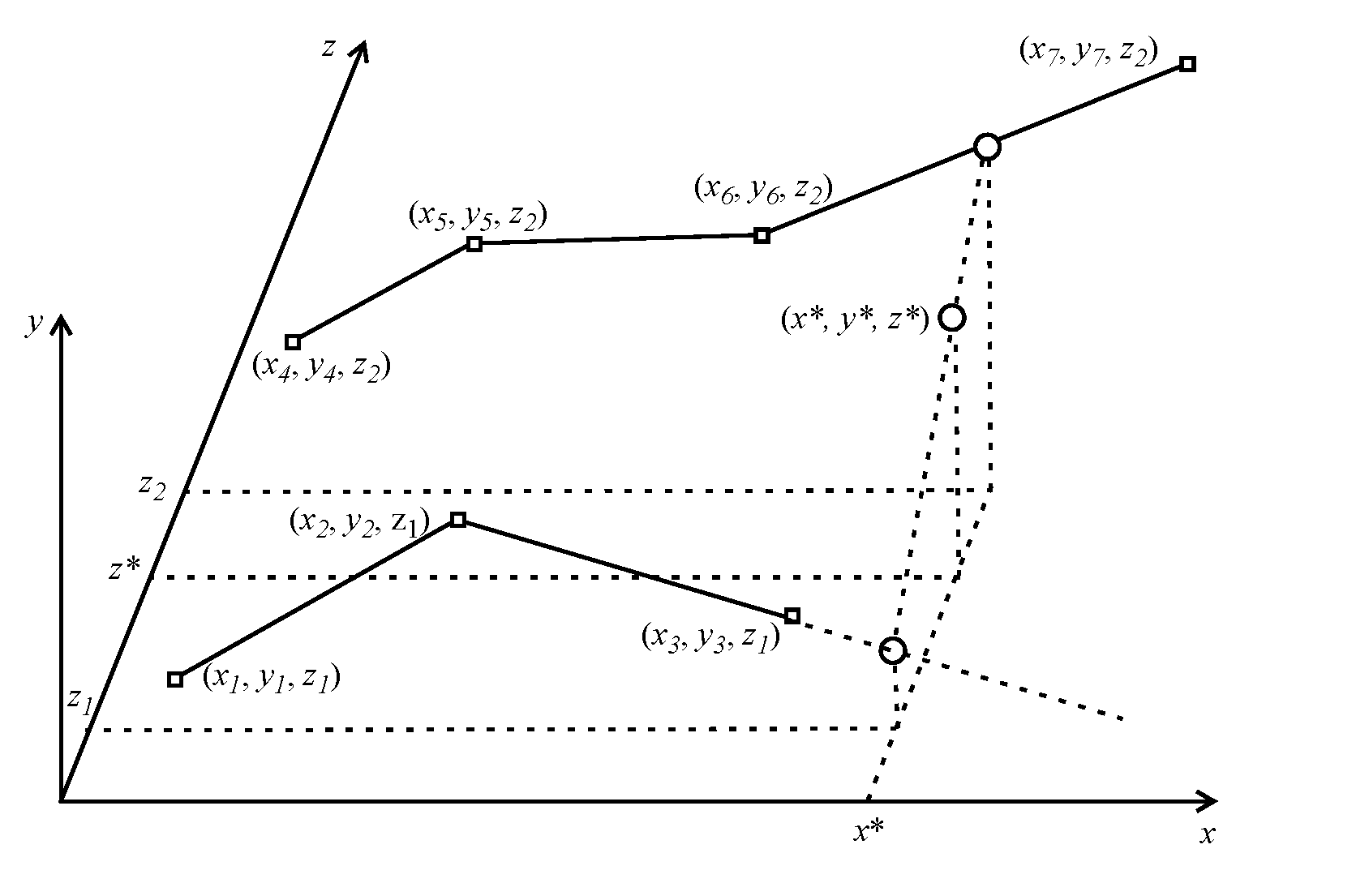
There is one special case in which the interpolation behavior is slightly different: when the x value being interpolated is within the domain of one of the bracketing constant z curves but not the other. In this case, we interpolate between the encompassing curve and the extrapolation of the other (shorter) curve. We extrapolate this curve with either the slope of its last segment or the slope of the corresponding segment of the encompassing curve, as appropriate for the particular table. To avoid overambitious extrapolation, RiverWare requires that the answer lie in the region bounded by the constant-z curves (that is, their convex hull). Figure B.3 illustrates this case, where the short curve is extrapolated with the slope of its last segment.
Figure B.3 Three-dimensional linear interpolation
Three-dimensional Table Interpolation Errors
The following types of errors may be reported during three-dimensional table interpolation:
• Invalid value (data error): an x, y, or z value is invalid (xi = NaN, yi = NaN, or zi = NaN for some i).
• Non-increasing z (data error): the z values are not increasing for one block to another (zi >= zi-1, for some i).
• Non-increasing x (data error): the x values are not increasing (xi >= xi-1, for some i).
• z value out of range (interpolation error): the z value being interpolated is out of the range of the table (z* < zmin or z* > zmax).
• x value out of range (interpolation error): the x value being interpolated is out of the domain of both of the two bounding constant z-curves.
Revised: 11/11/2019