
Release Notes Version 4.5
Special Attention Notes
• If the text or graphics in this file are not clear, you may need to print this document. Resolution should improve on the printed page.
• The new environment variable RIVERWARE_SITE has been added to specify the location of version-independent Riverware runtime files such as riverwareDB. Previously, the user had to copy their riverwareDB file to each new installation directory (specified by RIVERWARE_HOME). By setting the RIVERWARE_SITE environment variable to point to a new version-independent directory containing the user’s riverwareDB file, all future Riverware installations can automatically access these site-specific, version-independent runtime files.
RiverWare for Windows 2000 and Windows XP
RiverWare is available and supported for Windows 2000 and Windows XP (it will also run on NT but CADSWES is supporting Windows 2000 and XP). The user should be aware of the following differences that exist in RiverWare for Windows:
Differences in RiverWare for Windows
• Middle-mouse features such as QuickLink or rearranging the rows in the run analysis dialog are activated with the combination (pressed in this order): Alt + right mouse button + left mouse button. In Windows, the mouse configuration can also be changed so that middle mouse button actions are executed with the right mouse button (this would avoid the awkward sequence mentioned above).
• QuickLink can also be activated using the right-mouse button.
• The Windows DMI executable can be a DOS batch file or any other windows executable that can be run directly from a command shell.
Problems/Bugs in RiverWare for Windows
• The Locator View window often gets in a bad state when you resize the main workspace.
• It is possible that the objects may get shifted off the workspace if the workspace window is resized in certain ways. In order to make the objects visible again, you must save the model then reload it. Reloading the model will shift the model so that all objects are visible on the workspace.
Saving Model Files and Rulesets
• When saving model files or ruleset files that you intend to move between windows and unix systems, always save with the .gz extension. This saves the model/ruleset in a binary format that is the same on windows and unix.
General RiverWare
DMI
DMI File Chooser Path Is More Intuitive
The DMI file chooser path has been modified to open to the same path as the model file. After a selection has been made in the DMI file chooser, the file chooser will open to the last selected path.
DMI File Chooser “All Files”
In the DMI file chooser dialog, the "All Files" file chooser pattern was changed from "*.*" to "*" to include files without extensions. Now all files, with and without extensions, will be recognized by selecting "All Files".
SCT
The SCT 2.0 has been significantly enhanced. The enhancements to the SCT include new display features, new editing features, and new features related to open slot dialogs and printing. Other changes to the SCT include bug fixes. The general nature of these enhancements is described in the release notes below. More information on these enhancements can be found in Appendix 1: RiverWare 4.5 Release SCT Enhancements. The user is encouraged to consult the SCT 2.0 documentation in the User Interface section of the online help for a detailed description the general functionality of the SCT (not including these recent enhancements).
New Display Features
The SCT now supports optional day and year dividers (in addition to the month and weekend dividers that were already available). Slot dividers in the horizontal timestep orientation can now be made relatively thin- they used to always be tall enough to support a single line of text. Users can now select the font displayed in the SCT. The text color and background color of the Selection Info Area are also now user configurable. The horizontal timestep axis orientation now indicates when object dispatching has been disabled with red cross-hatching (this has always been the functionality in vertical timestep axis orientation).
User Settable Fonts
The user can now choose the SCT’s font. Only one font can be displayed at any given time and that font is used for both screen display and printing. Under the Font tab of the SCT Configuration dialog, the user can select one of three fonts, Default Font, Font A, and Font B. Under each of these items is a sample text field showing the font specification using the corresponding font. Under the Font A and Font B items are two buttons, Configure and Reset. The Configure button brings up the Qt Font Selector to allow the user to select a new font. The Reset button assigns the default font to the corresponding font item.
Editing Target Operations
It is now possible to edit/set target operations in the SCT even if the final timestep value of the target is NaN. If users set a target operation with NaN as the final value and then run the model, the run will abort as expected. For ease of editing, the SCT will no longer check this. Also, when setting values in a target operation with the SCT, values entered will automatically be entered in the final day of the target operation. When copying and pasting target operations, if the Target Begin timestep is not part of the copied region, the first timestep in the paste region will automatically be assigned the Target Begin flag.
Opening Multiple Slots Directly From the SCT
Users can now open multiple slots directly from the SCT by highlighting the desired slots and selecting the new "Slot->Open Slots" menu item. The toolbar button of a open folder is a shortcut to this operation.
Preservation of Height and Width
When an SCT is saved and reloaded, its width and height are now preserved.
Printer Properties
Individual use printer property choices for printing the SCT are now better preserved, particularly in situations where several users are operating RiverWare under the same login account.
Integrated Sum in Selection Info Area
The Selection Info Area at the bottom of the SCT has been enhanced to better support the summary of rate values (e.g., flow). When rate values are selected, the Integrated Sum of the values is displayed with an indication of the integrated unit type and unit (e.g., for "flow" values, the integrated unit type is "volume"). This is important primarily for irregular timesteps (e.g., monthly) for which the sum of various per-month rate quantities in differently-sized months is not well defined. Conventional summary information (e.g., Average, Min, Max, ...) of rates of irregular timesteps are based on the earliest timestep of the selection. The size of the irregular interval used in the calculation is indicated with the following nomenclature: /month28, /month29, /month30, /month31, /year, or /yearL (for leap-year).
Selecting Slots in New SCT
When starting a new empty SCT, a message box is displayed describing how to add Slots to the SCT and allowing the user to immediately open up either of the two Slot Selectors for that purpose.
Optional Date/Time Spinner
An optional Date/Time Spinner was added to the SCT for quick navigation to a particular timestep. The Date/Time Spinner can be optionally hidden or shown by the user with a new setting in the SCT Configuration dialog on the "Toolbar" tab.
General SCT Performance Enhancements
In the 4.4.0 release, having the SCT 2.0 open significantly slowed down Simulation and Optimization runs. This undesirable behavior has been fixed.
Previously, loading an SCT with multiple occurrences of the same slot, then loading a different SCT and then running a model was causing Riverware to become unstable. This problem has been fixed.
New Model Info Dialog
A new Model Info dialog has been added for storing users’ comments and a save history with the model file. This information is accessed by selecting "Model-> Model Info" from the main workspace menu. The File Info dialog box contains a "File Save History" field and a "File Comment" field. The File Save History field saves the user name, date, time, and version of RiverWare with which the model was saved. If a model is viewed and saved with RiverWare Viewer, the File Save History will indicate the model save information from the full version of RiverWare as well as model information from each save with RiverWare Viewer. Saving with the full (non Viewer) version of RiverWare will clear out the File Save History and only provide information about the most recent full version save. Saving with RiverWare Viewer will always append the File Save History field with the new save information. Note that the Model Info Dialog registers the save information only the first time you do a save during a RiverWare session. If you wish register the save in subsequent saves, you must choose the "Save As" option. (This functionality of the File Save History may be changed in future releases.) The File Comment field is an editable text field in which users can type any information or comments about the model. This information is stored with the model file. Users who plan to send copies of their models to RiverWare Viewer users will want to load and save their models with the most current release, and perhaps enter a brief description of the model in the File Comment field. This will provide RiverWare Viewer users with the appropriate model information.
Expression Slots
Expression slots have been significantly enhanced to offer more flexibility in editing and evaluation of expressions. The new expression slots, like the old expression slots, use a computational expression to specify how the values of a slot are computed. Existing expression slots will continue to work in RiverWare 4.5 however they will not be editable. If the user wishes to create a new expression slot or change an old expression slot, he/she will need to user the new expression slot editor. This editor uses RPL (RiverWare Policy Language) which is the same syntax used for writing rules. New functionality of the expression slots is outlined below:
Adding a New Expression Slot
The new expression slots are available on Data Objects by selecting Slot -> Add Series Slot with Expression or Slot -> Add Scalar Slot with Expression. Existing Expression Slots will continue to be supported, but users are encouraged to use the new scalar and series slot expressions to utilize the new functionality
Scalar and Series Expression Slots
Both scalar and series slots now may have their values computed by expression. Expression slots are identified by a ‘x’ in the upper right hand corner of the traditional scalar and series slot icons as shown:

Use of RPL
The computation of expression slots is now specified using RPL, the RiverWare Policy Language. RPL is computationally expressive and has an associated structured editor.
There is a special RPL set associated with RPL expression slots to which the user may add utility groups and functions. These functions may be called from any RPL expression slot.
Timing of Expression Slot Evaluation
The timing of expression evaluation is more flexible. The following options are available:
• interactively only
• beginning of the run
• end of the run
• beginning of the timestep
• end of the timestep
Users with large models might choose to evaluate expression slots interactively only, or at the end of run, to save on computation time. Evaluating expression slots interactively allows the user to select which expression slots to evaluate and these slots are evaluated only when the user chooses to do so. Users stepping through a model might choose to evaluate expression slots at the end of the timestep. Those interested in the final model result might choose to evaluate expression slots at the end of the run.
+ There is a special RPL set associated with RPL expression slots to which the user may add utility groups and functions. These functions may be called from any RPL expression slot.
Periodic Slots
Plotting
RiverWare 4.5 has the ability to add periodic slot curves to the plot dialog. The use of this feature should be fairly straightforward.
Multiple Year Periods
Multiple year periods are now supported on the Periodic Slot. The user can specify the number of years over which the data repeats. This is represented as year 1, year 2, year 3, ..., etc. with a user specified base year which represents the year at which the data cycle begins.
Data Objects
New Slots
Data objects have been enhanced to allow the additions of several new slots. The following slots can now be added to a data object: Series Slot, Series Slot with Expression, Aggregate Series Slot, Table Slot, Periodic Slot, Scalar Slot, and Scalar Slot with Expression. The new expression slots are a major enhancement and are described in more detail under the Expression Slots heading above.
Data Objects in Subbasins
Data objects are now allowed in user-defined subbasins.
Simulation Run Parameters
A few new features have been added to the Simulation Run Parameters dialog. This dialog is accessed by selecting View->Simulation Run Parameters from the main Run Control dialog. The first new addition is the Series Extension Increment field. This field has a default value of 1 but the user can increase this as necessary. This value tells RiverWare how much to extend a series slot if a value is written to a series slot at a date past the end of run date. For example, if the user changes the value from 1 to 10, then if a value is set past the end of run date on a series slot, that slot will be extended by 10 timesteps. This feature is useful only for performance improvement. If your model has very large series slots (many timesteps) and is often setting values past the end of run date on these slots (large lag times) then this value should be increased from 1 to the number of timesteps that represents the largest lag time.
The second new feature is a checkbox to model run analysis information. By default this is always enabled. If the user was not interested in seeing model run analysis information, he/she could disable this feature and may see a small performance improvement.
The third feature is a checkbox to enable the collection of RPL set performance information. This feature is disabled by default for performance reasons. If the user wanted to analyze the performance of any RPL sets (rulesets, expression slots, and user defined accounting methods), he/she could enable this feature and then analyze the data in the new RPL Analysis Dialog.
Extended Model File Precision
When saving a model file using the File->Save As menu option, the user now has the option to save the model data with extended precision. Normally all data is saved with 12 digits of precision. While this is enough precision for most applications, values that are saved to 12 digits of precision are not guaranteed to export and re-import as the same number (there may be differences in the last decimal place). Saving model data with extended precision will store values with 17 digits of precision. While this will increase the size of the model file, it will guarantee that all values are preserved when exporting and re-importing. The extended precision option is activated in the Confirm Save Model As dialog (the same dialog where you specify whether or not to save the model output). Once the extended precision option is activated, subsequent saves of that model will always save with extended precision.
Units
Units of “gal” (gallon) and “BG” (billion gallons)
The unit "gal" for "US liquid gallon" has been added to the RPLUnits (RiverWare Policy Language units) file. The unit "gal" will now be recognized in rulesets. The unit "gal" was already available for display in slots. The volume unit of "BG" (billion gallons) is now available in both Simulation and RiverWare Policy Language. For simulation, the slot configuration can be changed to display units of BG. For rules, the rule controller will now recognize and process rules with units of BG.
RiverWare Command Language (RCL)
A new command has been added to the RiverWare Command Language (RCL) used for running RiverWare in batch mode. An optional !SaveOutput flag has been added to the SaveWorkspace command if the user wants to save a model including the output data. If the model is configured to save the output already, then this flag is not necessary. However, the user may have the model configured to not save the output but may want to save the output when running the model in batch mode. The !SaveOutput flag would be necessary to accomplish that task.
RIVERWARE_SITE Environment Variable
The new environment variable RIVERWARE_SITE has been added to specify the location of version-independent Riverware runtime files such as riverwareDB. Previously, the user had to copy their riverwareDB file to each new installation directory (specified by RIVERWARE_HOME). By setting the RIVERWARE_SITE environment variable to point to a new version-independent directory containing the user’s riverwareDB file, all future Riverware installations can automatically access these site-specific, version-independent runtime files.
RiverWare Viewer
RiverWare Viewer is a new "read-only" version of RiverWare. This version of RiverWare is available at no cost to those who would like to view the output of model runs, but do not need to build, modify or run models themselves.
Current license holders do not need a new license to run RiverWare Viewer. Full RiverWare license holders can download the RiverWare 4.5 Release and run and examine RiverWare Viewer through the command line by typing:
riverware --viewer
Stakeholders and other parties interested in using only the RiverWare Viewer can download it for free from the CADSWES web pages. Information and instructions are provided on the RiverWare Viewer web page:
http://cadswes.colorado.edu/riverware/viewer/
RiverWare Viewer users must contact CADSWES directly for the free license file. In future releases, this process will be automated through the CADSWES web pages.
Simulation Objects
The following enhancements to the RiverWare simulation objects are described briefly. The user is encouraged to consult the Simulation Objects Documentation in the online help for more detailed descriptions of the enhancements to the objects and their methods.
Control Point Object
Flood Control Methods
The control point methods related to flood control were reorganized by adding a highest level category called Flood Control. This category serves to split the phase balancing (COE-KC) and operating level balancing (COE-SW) procedures. If users have existing models using flood control and control points, they will need to make the appropriate selection in the flood control category (from the default of None to one of the two flood control methods) to get back the related flood control categories. If the control point is a key control point, then the appropriate method in the key control point balancing category will need to be re-selected. Also the appropriate method in the regulation recession category will need to be re-selected if it was active prior to this release.
Additonal Peaking Flow Slot
A new slot, Additional Peaking Flow, was added to the Regualtion Discharge methods. Input to the new slot is optional and existing models do not require any changes. Additonal Peaking Flow is the difference between the estimated peak flow through the control point (average over the timestep) and the instantaneous peak during the timestep. Additional Peaking Flow is used in the empty space calculation. Empty space is calculated as the regulation discharge minus the inflow, minus the local inflow, minus the additional peaking flow (if a value is input). Typically, the Additional Peaking Flow slot will contain zeros for most timesteps and peak values on certain timesteps with peaks.
Reservoir Objects
Changes to Plant Efficiency Curve Power Method
The Plant Efficiency Curve Power Method on the Power Reservoirs has been changed. The method now generates the Auto Best Turbine Q Table using the second to last point in the Plant Power Table for a given operating head (previously, the second point was used). If there are only two points in the table for a given operating head, the second point is both the best efficiency and max capacity point.
The Plant Efficiency Curve Power method was new in the 4.4 release and allows the user to input several efficiency points instead of just the two (the best and max) available with the Plant Power Calc method. The Plant Power Table (a 3-D table that relates Operating Head, Turbine Release, and Power) is used to automatically generate the max and best turbine Q tables (called Auto Best Turbine Q and Auto Max Turbine Q) for this method.
Changes to Peak Power Calc and Peak Base Power Calc
In the PeakPowerCalc and PeakBasePowerCalc methods, if the Plant Power Cap Fraction was set to zero the Turbine Release was not automatically set to zero. Instead water was allowed to pass through the turbines instead of the spillways. Now, in both methods, if the Plant Power Cap Fraction is zero the Turbine Release is set to zero and any outflow is being correctly sent through the spillways.
Changes to Physical Constraint Methods (affects HypSim)
The physical constraint functionality was enhanced to eliminate problems associated with the hypothetical simulation functions. While this problem fixes some rare hypothetical simulation bugs, it could produce differences in the values returned by hypothetical simulation (especially when the outflow is at max capacity). The new code should improve the accuracy of hypothetical simulation but the user should be aware of possible model differences because of this.
Slope Power Reservoir
A new method category called Slope Partition was added to the Slope Power reservoir object. The new category contains the Partition BW Elevation method. This method allows the user to divide the reservoir into longitudinal partitions and calculate the steady flow through each partition (intermFlowParams). The flow parameter at each partition is then used in a 3-D table interpolation to find the backwater (BW) elevation at each of the partitions. This method does not affect the mass balance calculations and does not sum for the total storage over all partitions.
Stream Gage
Fractional Flow Method
The Stream Gage has a new method category, Conditional Flow Calc, that contains the Fractional Flow user method. The default method in this category is None, so existing models do not require changes. The new user method, Fractional Flow, calculates and sets Gage Inflow based on a comparison between two conditions. If Condition One is less than Condition Two, then the Gage Inflow is set to Condition One multiplied by a user input seasonal Loss Factor plus a user specified Constant. If Condition One is not less than Condition Two, then Gage Inflow is set to a user specified Normal Flow. The following pseudo-code displays the logic of how the Gage Inflow slot is calculated:
IF (Condition One (e.g., Diversion) < Condition Two (e.g., Diversion Requested))

ELSE
The Condition One, Condition Two, and Normal Flow slots can be user input, linked, or set by rules.
A new dispatch method solveGageInflowGivenConds sets Gage Inflow if the two dispatch slots Condition One and Condition Two are known. The gage object will dispatch using solveGageInflowGivenConds only if the user method Fractional Flow has been selected and neither Gage Inflow nor Gage Outflow are known. If the None method is selected, the Stream Gage does not dispatch. In that case, Gage Inflow and Gage Outflow are internally linked so values propagate immediately. This internal linking was the existing behavior on the Stream Gage.
Flood Control
Overview of Flood Control Algorithms
RiverWare has a new capability to execute basin-scale flood control algorithms on a computational subbasin. A flood control method is selected on the computational subbasin in the Flood Control method category. It is invoked by the new predefined rule function FloodControl(). Reservoirs and Control Points in the subbasin each have corresponding methods for flood control that should be selected consistently with the Computational Subbasin method.
Two Flood Control methods are available in this release. Both are basin-scale methods that calculate flood control releases from all reservoirs in the subbasin that are in the flood pool with the objectives of:
• maintaining a balance among the reservoir storages as prescribed by the specific method;
• avoiding flooding at downstream control points;
• calculating releases that empty the flood pools as soon as possible within a user-specified forecast period while maintaining constraints on increasing and decreasing releases.
Both the new Flood Control methods are based on US Army Corps of Engineers flood control algorithms. The Operating Balancing method is based on the Southwest Division SUPER program’s flood control algorithm. The Phase Balancing method is based on the flood control policy used by the Kansas City District. Both methods have been implemented in RiverWare as general methods that could potentially be used for flood control in any river basin. These Flood Control methods are still under development. Users who may interested in the new Flood Control methods should contact CADSWES before implementing them in their models.
A summary of how to use the new Flood Control methods is described in the next paragraphs. See the Simulation Objects Documentation and the Rulebased Simulation Documentation in the online help for details.
Model Configuration for Flood Control
In order to use the Flood Control methods, an existing RiverWare model should be configured as follows:
1. Add Control Point Objects to the points in the network where channel capacity limits the flood control releases.
2. Create a Computational Subbasin through the Edit SubBasins dialog on the Workspace menu. Include in the subbasin all objects that are part of the reservoir and river network, including the Control Points. All objects on the network must be linked and no loops may exist.
3. Select a Flood Control Method on the Subbasin. Select methods for all dependent method categories that appear when the Flood Control method is selected. Provide all input data required on the slots on the Computational Subbasin associated with the Flood Control method selected. See the Computational Subbasin Documentation for details about the methods and their input requirements.
4. Provide forecasted inflows (forecast the flood event). The inflows over the forecast period can be provided as Local Inflows to Reaches and Control Points and as Hydrologic Inflows to Reservoirs. You can forecast at some or all of these points. On each of these objects, select Forecast Local Inflows method under the Local Inflow Calculation or Hydrologic Inflow Calculation Category, then select the forecasting method you would like to use under the Generate Forecast Inflows Category. Provide data as needed to forecast the inflows at the control point. See each object’s documentation for details.
5. At control points, select the Regulation Discharge Method according to your policy. Select the Key Control Point Balancing method consistent with the Flood Control method you selected on the Subbasin and according to the regulation implemented at that control point. Flooding Exception and Sag Operation can also be selected. Provide input data as required for each method selection. See the Control Point documentation for details.
6. On Reservoirs, select the same method in the Flood Control Release Calculation category that you chose on the Computational Subbasin. Some data like forecast period can be propagated automatically to all reservoirs. See Computational Subbasin documentation for details. Provide data as needed by the method selected. See specific Reservoir object documentation for details.
Note: Sloped Storage Reservoirs cannot be included in a subbasin using the current selection of Flood Control methods because both methods require a unique relationship between Storage and Pool Elevation.
7. On Reservoirs, select a method for Surcharge Release. This method releases water in the Surcharge Pool that is not subject to downstream channel constraints. Provide data as needed by the method selected. See the Reservoir object documentation for details.
Execution of Flood Control Algorithm in Simulation
The new flood control algorithms are designed to be executed by rules. Following is a description of how the many parts of the flood control algorithm are executed in order at each timestep. See the documentation for each object for further details.
• During execution of the Beginning of Timestep routines on the Reservoir, Control Point and Reach objects, the selected Inflow Forecasting methods are executed, setting the Hydrologic Inflow Forecast slot for all timesteps in the Forecast Period, beginning with the current simulation timestep. The objects do not dispatch as a result of the setting of the Hydrologic Inflow slot.
• Lower priority rules execute and simulation propagates the results until the flood rules are next on the agenda.
• The first set of flood rules to execute sets the Surcharge Release Flag (S) on the Outflow slot of each Reservoir in the computational subbasin. A separate rule sets the Surcharge Release Flag on each Reservoir starting with the upstream reservoirs and continuing downstream. The simulation after each rule execution dispatches the Reservoir. The Surcharge Release Flag is interpreted as an input, so the reservoir executes the solveMB_givenInflowOutflow. As the dispatch method is being executed, the Surcharge Release Flag is detected and the object executes the selected surcharge release method. The surcharge releases are computed for the entire forecast period. These surcharge releases are set in the surcharge release slot. Also, the outflow slot is set equal to the surcharge release slot. After surcharge calculations are completed, the Surcharge Release Flag is removed from the current controller timestep so that surcharge releases will not be recomputed on subsequent dispatches. When the reservoir solves, it routes its surcharge releases down to the next reservoir before it (the downstream reservoir) computes surcharge releases.
• The next rule sets the Regulation Discharge (G) flag on the Reg Discharge Calculation slot on each Control Point in the Computational Subbasin for the current timestep. Setting this flag results in execution of the dispatch method which in turn executes the selected Regulation Discharge method and any dependent methods (such as Balance Level) on the Control Point. After execution, the regulation discharge flag is removed so that regulation discharge will not redispatch unless this flag is reset by a rule. After executing the selected Regulation Discharge method, the dispatch method checks to see if outflow has changed from its previous value. If it has not, the outflow slot is not reset using the regulation discharge rule priority. This prevents the regulation discharge rule priority from propagating downstream and triggering unnecessary and, in some cases, undesirable resolving.
• Lastly, a single rule invokes the predefined FloodControl() function on the subbasin. The function executes the selected Flood Control method on the Computational Subbasin. The function returns values for Outflow and Flood Control Release for each reservoir in the computational subbasin at the current controller timestep. The rule then sets the Flood Control Release and Outflow slots on each reservoir (outflow is the sum of flood control release and surcharge release). The setting of outflow triggers each reservoir to dispatch with the solveMB_givenInflowOutflow dispatch method. Nothing out of the ordinary happens in the dispatch method as a result (it doesn’t matter that we’re dispatching as a result of flood control, the object dispatches as it normally would when getting a new outflow).
Rulebased Simulation
RPL Analysis Dialog (“Rule Calling Tree”)
The new RPL Analysis Dialog is a tool for analyzing and documenting a RPL set. This highly customizable dialog displays detailed information about all objects in a RPL Set (including descriptions and performance information) and the relationships between these objects. Below is a brief description of the RPL Analysis Dialog.
This new dialog is available from any RPL editor dialog by selecting Ruleset->Ruleset Analysis....
Detailed documentation on the use of the RPL Analysis Dialog can be found in the online help under Rulebased Simulation Documentation. Some key features of the new RPL Analysis Dialog are described below:
• + Three synchronized treeviews onto the entire ruleset:
– 1) the classic groups view
– 2) descending the static call graph (displays which functions are called by an object)
– 3) ascending the static call graph (displays which functions call an object)
• + Selecting an object in one view automatically selects and scrolls to the same object in the other views)
• + Displays information and relationships between any user-selectable object types, including: statements, predefined functions, rules, etc.
• + User-customizable column types, including object descriptions and performance information.
• + Opens any RPL editor dialog, including "Replace existing editor" mode where opening a new dialog closes the previously opened dialog to avoid screen clutter.
• + Allows printing and exporting (tab-delimited text files) of any portion of the views.
• + Navigation shortcuts for each treeview.
New Palette Buttons for Set Operations (where lists are sets)
Union
The set union expression takes two lists and returns a single list that contains the items that are in either list or both lists. Duplicate items are removed.
Intersection
The set intersection expression takes two lists and returns a single list that contains the items that are in both lists.
<L> - <L> Set Difference
The set difference expression takes two lists and returns a single list that contains the items that are in the left hand list but not in the right hand list.
<L> ^ <L> Set Symmetric Difference
The set symmetric difference expression takes two lists and returns a single list that contains the items that are not in both lists. This is equivalent to the expression:
(list1 U list2) - (list1 intersect list2)
This is also equivalent to the expression:
(list1 - list2) U (list2 - list1)
Rules Palette Predefined Functions
Following is a brief description of new predefined functions and changes to existing predefined functions available for use in the RiverWare Policy Language. Details on the use of these functions and the syntax involved are available in the Rulebased Simulation Documentation in the online help.
Modified Predefined Functions
The following predefined functions have been modified to return the account names in ascending priority date order:
AccountNamesByAccountType
AccountNamesByWaterType
AccountNamesByWaterOwner
AccountNamesFromObjReleaseDestination
AccountNamesFromObjReleaseDestinationIntra
(Previously these predefined functions returned the account names in alphabetical order, though this behavior was not a documented feature.)
Slot Sum Functions Now Accept Periodic Slots
RiverWare 4.5 supports periodic slots as arguments to RPL predefined functions which, in prior releases, only supported series slots. Where appropriate, RiverWare uses lookups on the periodic slot at dates in synch with the run series. The following predefined functions were enhanced to work for periodic slots: SumFlowsToVolume, SumFlowsToVolumeSkipNaN, SumSlot, SumSlotSkipNaN, GetSlotVals, GetDisplayVal.
Since Periodic Slots often have multiple columns, new predefined functions were added to sum slots or get slot values by column: SumFlowsToVolumeByCol, SumFlowsToVolumeByColSkipNaN, SumSlotByCol, SumSlotByColSkipNaN, GetSlotValsByCol, GetDisplayValByCol. These functions can also be used to sum columns on Aggregate Series slots.
AccountPriorityDate (STRING AccountName)
This function accepts one STRING argument, an account name, and returns a DATETIME, the account’s priority date. The function fails if the account doesn’t exist or if it doesn’t have a priority date. (PassThroughAccounts do not have a priority date; StorageAccounts and DiversionAccounts have a priority date if the user specified one in the user interface.)
AccountNameFromPriorityDate (DATETIME PriorityDate)
This function accepts one DATETIME argument, a priority date, and returns a STRING, the name of the account with the priority date. The function fails if no account has the priority date.
Note that the two new predefined functions described above can be used with the existing Maplist predefined function to map a list of account names to a list of priority dates, or a list of priority dates to a list of account names.
SortPairsAscending (LIST pairs) SortPairsDescending (LIST pairs)
The input LIST, pairs, must be a list of lists and each member list must contain at least two elements. The pairs are sorted into ascending/descending order by the second element’s value and a list containing the first elements of this sorted list of pairs is returned. Duplicates are not removed.
Sort (LIST)
This functions sorts a list into increasing order.
Reverse (LIST)
This function reverses the order of items in a list.
GetDate (STRING dateText)
This function returns the date which corresponds to the input text. Legal text is the same as is legal for symbolic date/times. In other words, it takes a STRING and turns it into the corresponding DATETIME. For example, the expression
GetDate(“January 1, Current Year”)
is exactly equivalent to the expression
@“January 1, Current Year”
SolveOutflowGivenEnergyInflow
This function returns the outflow of the specified reservoir given a value for energy and inflow.
Inline Comments in Rules
Rulesets (and all other RPL sets) have been enhanced to allow inline comments. Two new buttons have been added to the RPL Palette: Add Comment and Delete Comment. These features are used to add or remove a text comment from the body of the rule or function.
Printing Rulesets
The dialogs used to print RPL sets have been re-implemented in Qt. As part of this work new printing options and features have been made available. Information is available in the online help under Rulebased Simulation Documentation if more detail is required on printing and formatting RPL sets.
Accounting
Automated Pass Through Account Creation Function
It is now possible to automatically generate pass-through accounts. This function allows the user to identify two existing accounts on different simulation objects and create linked pass-through accounts on all intermediate simulation objects in one single operation. This new functionality is a convenient alternative to creating pass through account via the Open Object dialog individually for each intermediate object. The Pass Through Account Creation dialog can be accessed from either the Open Object dialog box or the Water Accounts Manager dialog box. From either of these dialogs select Account -> Create -> Pass Through Accounts. Next, select the desired upstream account and desired downstream account. Select or enter the desired Account Name, Account Water Type, Account Water Owner, Supply Release Type, and Supply Destination. Select OK and all intermediate pass through accounts will be automatically generated. Further details on the Automated Pass Through Account Creation Function are available in the User Interface section of the online help.
Account Manager Dialog
Several new capabilities have been added to the Account manager Dialog. During this enhancement process, the Accounting Manager dialog box was ported from Galaxy (GUI toolkit) to Qt.
A new property, Account Priority Date, can be now be set via the Account Manager Dialog box. The Account Priority Date represents the date a water right was acquired and can be set on Storage and Diversion Accounts. Priority date is specified by Year, Month, Day, and hour (1 to 24). No two accounts may have the same Account Priority Date.
It is also now possible to set the Water Type and Water Owner of multiple Accounts via the Account Manger Dialog. Note that properties can not be set on accounts having an open Account Configuration dialog -- a warning message pop-up dialog informs the user of that condition, and allows the user to raise the Account Configuration dialog box.
More information is available in the User Interface section of the online help.
Supply Manager Dialog
The RiverWare Supplies Manager can now show and sort Supply Types. The Supplies Manager dialog box shows a single Supply per row. There are two configurable data columns which can each show one of several properties of the Supply or of the Supply’s Upstream or Downstream Account. ("Supply Type" was just added to the available selections). The Supply Types are indicated with these names: ST_DivRet, ST_InOut, and ST_Transfers.
More information is available in the User Interface section of the online help.
Priority Date Fields
Accounts now have an optional attribute called Priority Date. An account can be configured to have a priority date through either the account configuration dialog (to modify a single account) or through the Water Accounts Manager dialog. The priority date is used to specify the priority of an account. An earlier priority date implies a higher priority. This information can be used to sort accounts by priority date in the Water Accounts Manager dialog, or it can be used in conjunction with the new RPL predefined functions that make use of this information. These functions are discussed in the Rulebased Simulation section above.
Plotting Account Multislot Data
RiverWare now supports plotting of account data at both the account level and the multislot level. If the user has an account open, a slot can be plotted by selecting a column and selecting the plot menu item (under the File menu title). In addition, if the user double-clicks on a multislot (i.e. Outflow or Inflow) to open the multislot detail dialog, the user can plot the data from individual supplies by selecting a column and using the plot menu item.
Optimization
Diagnostics
New Diagnostic reports in millions of dollars
A new optimization diagnostic reports the final objective function value in millions of dollars.
Warning Messages Removed
The warning messages informing users that they have created additional optimization variables have been removed. User-created optimization variables are now available for AggSeries slots and are the recommended option for user-created variables. These slots function approximately the way Outflow slots on reservoirs do. They automatically add columns for a total of 3 columns. The optimization output column is copied over to the simulation column and is marked as input. When the next optimization run starts all, the values in both the simulation and optimization output columns are cleared.
Power Regulation
Hydropower can be an economic source of ancillary power services. One ancillary service, power “regulation”, uses hydropower to “follow” fluctuations in real-time power demand. With this release, RiverWare has methods which allocate turbine capacity for power regulation. After modeling is complete, the allocated capacity becomes available to dispatchers for real-time load following.
This functionality is intended to be used primarily with optimization and post-optimization simulation in RiverWare. Consequently, most non-optimization users will not want to model power regulation and the default settings for the methods related to power regulation reflect this. On power reservoirs, the new method category is “Regulation Category”, and the default setting is “None”.On thermal objects, the new method category is “Regulation”, and the default setting is “No Regulation”.
Detailed documentation on how optimization users can add regulation to their models is in the document, Power Regulation in RiverWare, available from CADSWES.
Objective Function
Thermal Object Avoided Operating Cost
When optimization reports an objective function value that includes "Thermal Object.Avoided Operating Cost" the units will now be reported in the units selected by the user for the "Thermal Object.Total Values" slot.
Thermal Objective Reported in Simulation
Simulation has a new method category, "Thermal Objective Reported", that controls which objective is reported for simulation. At this time there are four methods that use the existing slots:
1. none
2. Avoided Cost
3. Avoided Cost Plus Cumulative Value of Storage (includes the value of final storage)
4. Avoided Cost Plus Net Cumulative Value of Storage (includes final value - initial value)
The units for the Total Value slot will also be used for reporting this value.
SCT
New Display Features
Optional Day and Year Dividers
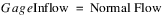
The original release of SCT 2.0 supported optional automatic divider rows and columns for months and for weekends (between Friday & Saturday, and between Sunday & Monday). The new release also supports optional automatic divider rows and columns for days and years. Each of these four types of time dividers can be independently enabled or disabled, and can be shown with independently configurable colors.
To configure these options, select “View >> SCT Configuration ...” menu item, and operate these controls of the indicated tabbed panes:
“Horz Time” tab (see image -->)
• [ ] Draw Day Divider Columns
• [ ] Draw Weekend Divider Columns
• [ ] Draw Month Divider Columns
• [ ] Draw Year Divider Columns
“Vert Time” tab
• [ ] Draw Day Divider Rows
• [ ] Draw Weekend Divider Rows
• [ ] Draw Month Divider Rows
• [ ] Draw Year Divider Rows
“Color” tab (press the buttons to pick a different color)
• [ ] Day Divider
• [ ] Weekend Divider
• [ ] Month Divider
• [ ] Year Divider
Textless, Thick-Line Slot Divider Option in Horizontal Timestep Axis Orientation
The user can insert “slot dividers” in between slot rows or slot columns. In horizontal timestep axis orientation (where slots correspond to rows), slot dividers were originally made tall enough for a single line of text. Now, there is an option to draw slot divider rows as only a thick colored line.
This option is selected for the whole SCT. That is, all slot divider rows (in horizontal timestep axis orientation) can be either tall enough for text labels, or can be drawn as only a thick horizontal line. This selection is made by the user in the “Horz Time” tab of the SCT Configuration dialog box with the following new toggle button:
• [ ] Text Labels in Slot Divider Rows
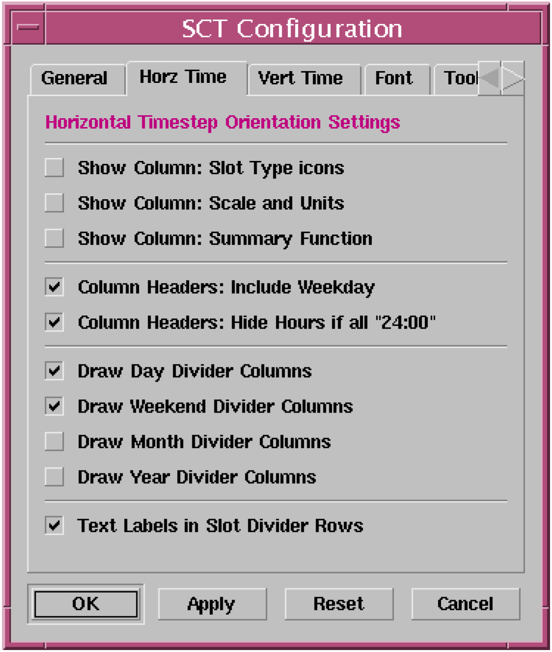
User Settable Fonts
The user can choose the SCT’s font. Only one font can be displayed at any given time, and that font is used for both screen display and printing.
Two custom font specifications can be saved with each SCT, and with the default SCT configuration. The user can choose to use either of those two custom font specification, or the default font.
To choose between those three options (Default Font, Font A and Font B), and to configure the font specification for the latter two options, open up the SCT Configuration dialog box by selecting the “View >> SCT Configuration ...” menu item, and select the “Font” tab.
Select one of the three radio buttons to indicate the font specification to be used by the SCT.
Select either of the “Configure” pushbuttons to change the corresponding custom font specification. This brings up a font selector which allows the user to select a different font face (font family), font size, font weight (e.g. normal or bold), and other font properties.
Select either of the “Reset” buttons associated with either the Font A or Font B item to restore that font specification to the default font.
Applying a font specification to the SCT (with either the “OK” or “Apply” button) may take a moment to complete since the SCT’s geometry needs to be readjusted.
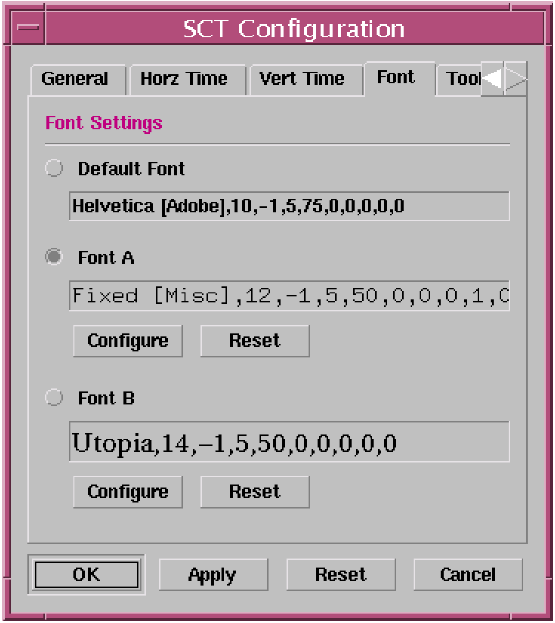
Selection Info Area: User Settable Background and Text Colors
The user can now configure the colors for the Background and the Text displayed in the Selection Info Area at the bottom of the SCT. These colors are chosen from the “Summary” panel of SCT Configuration Dialog Box. Pressing either of these buttons brings up a Color Chooser:
Selection Info Area
• [ ] Text Color
• [ ] Background Color
See image to the right and in the next section.
Selection Info Area: Integrated Sums for “per-time” values (e.g. Flow)
When values of only one particular RATE ("per-time") unit type are selected, the "Integrated Sum" of those selected values is displayed, with an indication of the integrated unit type and unit (e.g. for "flow" values, the integrated unit type is "volume" -- and for “power” values, the integrated unit type is “energy”). See the image below.
This is important primarily for irregular timesteps (e.g. monthly) where the sum of various per-month rate quantities in differently-sized months isn’t well defined. The integrated value is also useful where the rate values’ display-unit time component differs from the timestep (e.g. cms values in a daily timestep model).
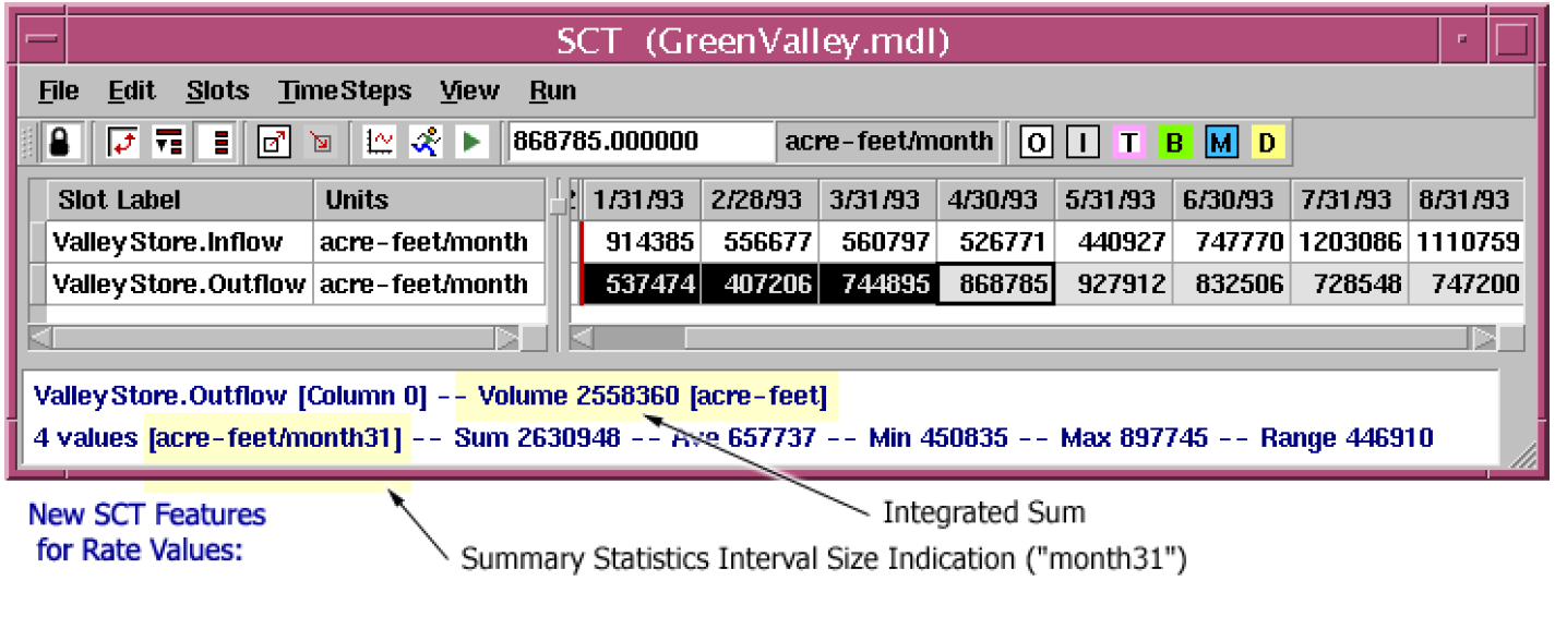
Selection Info Area: Interval size indication for irregular time units (e.g. monthly)
Apart from the Integrated Sum described in the previous section, the display of conventional summary statistics (e.g. average, minumum, maximum) of a selected set of irregular rate values is enhanced. All summary computations are done in well defined rate units (e.g. something per-second). But the user can choose to have rate values displayed in “per-month” or “per-year” values -- which are not generally well defined over multiple months or years. To address this ambiguity, the KIND of month or year which is used to convert the computed summary statistics is indicated in the Selection Info Area using the following nomenclature, (see also the image above):
... /month28
... /month29
... /month30
... /month31
... /year
... /yearL
The particular interval used for that conversion is based on the size of the earliest timestep in the selection.
Object Dispatching Ornamentation in Vertical Timestep Axis Orientation
To indicate that a slot’s object’s dispatching is disabled, the original release of SCT 2.0 supported a crosshatch ornamentation drawn on slot labels only in horizontal timestep axis orientation (where rows correspond to slots). There was no such ornamentation implemented for vertical timestep axis orientation (where columns correspond to slots). Now, in that orientation, the crosshatch for such slots (whose object’s dispatching is disabled) is drawn over the data cells, using the same user defined color for the object dispatching crosshatch. [The omission of this feature in the original SCT 2.0 release was documented as bug 3431].
New Editing Features
Changes to Target Operation Editing
1. Target Operation: No restriction on final timestep value for Setting a new Target Operation
The “Edit >> Target Operation” menu item and the Target Operation toolbar button used to be unavailable to the user (disabled) if the final timestep of the current cell selection didn’t have a defined numeric value. Now, the availability of that operation (to create a new Target Operation) is not dependent on the final timestep numeric value. Any Target Operation having an undefined (“NaN”) value in the final timestep will cause a model run failure, but the user is no longer prevented from creating it. The user must enter a value in that final timestep for the Target Operation to become valid. Note that selecting the final timestep cell of a defined Target Operation and entering a value will preserve the Target flag on that timestep.
2. Target Operation: Setting a Target Operation results in giving Keyboard Input Focus to the final selected timestep.
The typical way of defining a new Target Operation is to first select the range of timesteps within a Reservoir Storage or Pool Elevation Slot, and either select the “Edit >> Target Operation” menu item or press the Target Operation toolbar button. Before this feature was revised, the selection of that whole timestep range remained -- so any subsequent entry of digits caused every timestep within the new Target Operation to be assigned the entered value. This behavior was revised. Now, as a result of defining a new Target Operation, keyboard focus is forced to the final timestep in the selected range. Subsequent entry of digits causes the assignment of the entered number to only the final “target” timestep.
3. Target Operation: Copying of incompletely selected Target Operations
The original release of SCT 2.0 didn’t paste a Target Operation to the destination timesteps if the originally selected source (copied) timesteps didn’t include both the Target Begin and Target (End) timesteps. (But this limitation applies only to Target Operations that include a Target Begin timestep, and not those defined with only a Target [end] Flagged timestep).
With the revised SCT, if the copied region contains a Target (end) Flag, but not a corresponding Target Begin Flagged timesteps (and if this is a Target Operation which actually does have an explicit Target Begin Flag), then a Target Operation is defined in the destination (paste) timestep region, with the Target Begin Flag assigned to the earliest timestep in that destination timestep region.
Note that if a single timestep is selected as the destination region (for the paste operation), then that timestep is effectively the first timestep of an implied multiple-timestep destination region which is the same size as the original source (copied) timestep region. So, in the scenario described above, that single selected destination region would receive the Target Begin flag.
Other New Features
Open Slot Dialogs shown from the SCT
Open Slot dialog boxes for simulation slots (and not for accounting slots) can now be opened from the SCT. When one or more slots are selected, selecting the new “Slot >> Open Slots ...” menu item or the new Open Slots toolbar button (see the following image) the Open Slot dialog boxes for the selected slots are shown. If Open Object dialog boxes for those slots are already open (e.g. previously opened from the Open Object dialog box), then those existing Open Slot dialog boxes are raised.

As with most of the other toolbar buttons, the Open Slot toolbar button is optionally shown. To show or hide this new toolbar button, select the “View >> SCT Configuration ...” menu item and select the “Toolbar” tab. Select or deselect this toggle button:
[ ] Button: Open Slots
Window Size Persistence
When an SCT is saved and reloaded, its width and height are preserved. This is automatic -- no user operations or settings are required.
When the user saves the current SCT as the default SCT configuration (with “View >> Defaults >> Save Current Settings as Default”), the current size of the SCT becomes the default SCT size.
The default SCT configuration is used in these three situations:
when a new SCT is created;
when the user migrates an old SCT (1.0) to the new SCT;
when the user applies the default configuration to an SCT using “View >> Defaults >> Apply Default Settings”.
Printer Settings
The original release of the SCT 2.0 read and saved the printer selection and printer property choices with every print operation. These values are saved in the “user preferences” of the currently logged-in user account. This causes a problem for RiverWare users who are sharing a single Unix (Solaris) user account. Now, those values are read from the user account preferences only at RiverWare program startup, and are saved at RiverWare program exit (but only if the print operation was used during the session). This insures that a particular person’s print selections remain stable during a RiverWare session even if other users are operating RiverWare logged in under the same user account.
Optional Date/Time Spinner for Timestep Navigation
An optional Date/Time spinner was added to the SCT 2.0 Toolbar for navigating (automatically scrolling) to specified timesteps. This will be useful especially in models with many timesteps.
The Date/Time spinner can be shown or hidden by the user, depending on a setting in the SCT Configuration which is stored in SCT files. The low-level default is to SHOW the DateTime Spinner. (That default can be changed by hiding the DateTime Spinner in an SCT, and then saving that SCT configuration as the default configuration with "View >> Defaults >> Save Current Settings as Default").
To Show or Hide the DateTime spinner:
Select from the SCT menubar: "View >> SCT Configuration ..."
Select the "Toolbar" tab
Turn on or off the following toggle button: [X] Date Time Spinner
Select the [OK] or [Apply] buttons.
Entering a date in the Spinner, or operating the up and down buttons of the Date/Time spinner causes the SCT to be scrolled horizontally or vertically (depending on the timestep axis orientation) so that the indicated timestep is shown in the leftmost column or topmost row. An exception to this is when the indicated timestep is within the last "screen" of the time range, in which case the SCT is just scrolled to that last screen.
The Date/Time spinner’s up and down buttons change the indicated date/time by one timestep, even when the SCT is showing timestep aggregations. Since all the timesteps within an SCT timestep aggregation are shown within the same column (and row -- when details are hidden), the SCT will not always be scrolled as a result of clicking the spinner’s up and down buttons.
The "step" of the Date/Time spinner matches the Run Control timestep interval. The Date/Time spinner’s time range matches the SCT’s time range, which is the time range of Run Control PLUS the number of visible PRE-simulation and POST-simulation timesteps configured in the SCT.
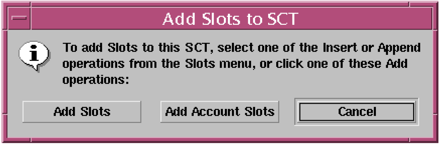
Opening a new SCT, prompt to Add Slots
When creating a new SCT, the message box illustrated below is presented to the user for easy initiation of Slot Selection to add Slots to the SCT. This occurs only if the Workspace is not empty (i.e. only if at least one Object exists).
SCT Bug Fixes
Selection Info Area: “Obscured Timesteps” Description on Summary Cells
The time range of certain Series Slots may extend beyond the time range of the SCT. When this occurs, a corner triangle ornament is shown in the upper left or lower right of the slots’s first or last timestep cell. Actually, this is shown on both summary cells and detail cells. When one of those cells is selected, a message is displayed in the SCT selection info area (at the bottom of the SCT) indicating the number of timesteps of the Slot which are not visible (i.e. the number of “obscured” timesteps).
There was a bug which sometimes prevented the display of that information in the selection info area when a summary cell was selected. This is now fixed.
Target Operation setting operation: Expand slot’s time series
Setting a Target Operation failed (had no effect) if the selected timestep cells extended before or after the time range of the slot. That time range is now expanded as needed.
SCT Configuration Dialog Box fixes
(A) The SCT Configuration dialog box has both an “OK” button and an “Apply” button which apply the user’s settings to the SCT. The “OK” button performs the “Apply” operation and dismisses the dialog box. There was a bug which sometimes prevented the “OK” button to apply changes if the “Apply” button had previously been operated. This is now fixed.
(B) Applying changes made in the SCT Configuration dialog box interfered with other changes to the SCT (e.g. swapping axis or changes to the timestep aggregation configuration) made when the SCT Configuration dialog box was already open. This is now fixed.
Selection Information Area: Read Only
The Selection Information Area at the bottom of the SCT had been editable by the user. That is now disabled, but the user can still copy text from that area by (1) selecting the desired text, (2) pressing the right mouse button over the selected text, and (3) clicking “Copy” from the context popup menu.
Saved “Lock” status not staying locked on loading an SCT from the Workspace.
The SCT supports a “Lock” toggle which allows certain aspects of the SCT configuration -- generally the set of slots represented in the SCT and the labels used for those slots -- to be unchangeable. With the original release of the SCT 2.0, an SCT opened from the RiverWare workspace always came up UN-locked, regardless of the lock status of the saved SCT. This is now fixed.
Retaining window scroll position after adding slots and other reconfigurations.
With the original release of the SCT 2.0, the action of adding or inserting slots, or performing many other reconfigurations caused the SCT to redisplay from the top-left corner.
Now for slot / slot divider insertion operations and most configuration change operations, the SCT scroll position is retained (measured in pixels from the top-left). An exception to this is the slot append operation, which causes the SCT to redisplay at the end of the slot list (either the last row or the last column, depending on the timestep axis orientation).
Target Operation: Invalid state possible when pasting a new target operation over an existing one.
Bug 3446. Under certain conditions, as a result of pasting a copied timesteps containing a target operation, it was possible for the Begin Target flag of an existing Target Operation to not be cleared when it should have been. This is now fixed.
Model name change not reflected in SCT window title.
Bug 3435. The SCT window title shows both the name of the SCT and the name of the currently loaded model. The latter was not being updated when the name of the loaded model (i.e. the name of the RiverWare workspace) was changed, e.g. after performing a “Model >> Save As ...” operation from the workspace window. This is now fixed.
Selecting OK in the Multiple Slot Selector does not always add the highlighted slots to the SCT.
Bug 3432. There were actually several bugs in the Multiple Slot Selector, including a related one which showed up in the Diagnostic Manager (See bug 3526 and 3533 in the bug reporting system -- not described in this document).
Disable Dispatching cross-hatching is not updated in the SCT when selected from the Model Run Analysis dialog.
Bug 3433. Before the SCT 2.0, the Model Run Analysis dialog was the only place from which the Object Dispatching Disabled state for an Object could be changed, so no system-wide notification was needed, and none was implemented. This has been added. So any change of this property on an Object made in any SCT or in the Model Run Analysis dialog now causes an update in the others displaying the respective Object.
Bad Timeslice copying: Paste as Input into TableSeriesSlots
Bug 3498. When copying a whole timestep range across all Slot Items in an SCT which includes Table Series Slots, the Paste As Input operation skipped every other target timestep. For example, for a Table Series Slot:
• Selected Values: 111 222 333 444
• Target Values: 111 (no change) 222 (no change)
Can’t see data in high precision in SCT
Bug 3512. The contents of the Toolbar Value Entry Field and the initial value displayed during an in-cell edit operation had been displayed always with six fractional decimal digits, regardless of the configured “precision” of the Slot containing the value. Now, the Slot’s precision is respected, but a minimum of six fractional decimal digits are displayed.
Slot name changes not handled properly.
The association between an SCT’s reference to a Slot and the actual Slot wasn’t being maintained when the Slot’s name changed. A Slot’s name can change in the following three ways:
The Slot’s containing Object is renamed by the user.
The Slot’s containing Account is renamed by the user.
For Slots on a Data Object, the Slot is renamed by the user.
The change of a Slot’s name doesn’t effect the displayed Slot item label, since the Slot label is only initialized from the Slot name. But the Slot List saved in SCT files, and the display of the actual Slot name in other parts of the SCT (e.g. in the Selection Info area) do need to use the actual current Slot name.
Bug Fixes
The following is a list of the bugs which were fixed for this release. If you wish to view the details for a specific bug, please browse to http://cadswes.colorado.edu/users/gnats-query.html and search our bug database. You will need a RiverWare user login and password.
351 | 431 | 447 | 494 | 593 | 599 | 663 |
739 | 781 | 967 | 1184 | 1607 | 1824 | 2553 |
2573 | 2590 | 2639 | 2670 | 2851 | 3068 | 3115 |
3116 | 3261 | 3349 | 3352 | 3381 | 3396 | 3396 |
3400 | 3401 | 3402 | 3403 | 3404 | 3405 | 3407 |
3408 | 3409 | 3410 | 3411 | 3415 | 3416 | 3418 |
3420 | 3421 | 3422 | 3423 | 3424 | 3426 | 3427 |
3428 | 3429 | 3431 | 3432 | 3433 | 3434 | 3435 |
3436 | 3437 | 3438 | 3439 | 3440 | 3442 | 3444 |
3445 | 3446 | 3447 | 3448 | 3449 | 3450 | 3451 |
3452 | 3453 | 3454 | 3455 | 3457 | 3458 | 3459 |
3461 | 3462 | 3463 | 3465 | 3466 | 3467 | 3468 |
3469 | 3470 | 3471 | 3472 | 3473 | 3474 | 3475 |
3476 | 3477 | 3479 | 3480 | 3482 | 3483 | 3483 |
3484 | 3485 | 3486 | 3487 | 3488 | 3489 | 3493 |
3494 | 3497 | 3498 | 3499 | 3500 | 3503 | 3506 |
3508 | 3512 | 3513 | 3515 | 3516 | 3517 | 3518 |
3521 | 3522 | 3524 | 3525 | 3526 | 3528 | 3529 |
3530 | 3533 | 3539 | 3540 | 3541 | 3543 | 3546 |
Revised: 11/11/2019