
Optimization
Spill Computation Methods
A new User Method Category called Optimization Spill Computation has been added to all Reservoir objects. This Category is only available when the independentLinearizations Method is selected in the Optimization Power Computation Category. The Optimization Spill Computation Category contains six Methods for the linearization of spillway physical constraints. The selected Method should reflect the number and types of spillways being modeled and must be the same as the selected Method in Simulation. The physical data for all selected spillways is combined into a single Storage vs. Spill table. This table is then linearized according to the linearization Method selected in the Spill Lower Bound MTLE Category and the Spill Upper Bound MTGE Category. The available Methods for the Spill Lower Bound MTLE Category are Piecewise and Line. The only available Method for the Spill Upper Bound MTGE Category is Line.
All of the Methods solve by generating a composite Spill Bounds Linearization Table from the points in the Unregulated, Regulated, and/or Bypass Spill Tables. The first column of the Spill Bounds Linearization Table contains monotonically increasing Storage values. These values correspond to the combined set of Pool Elevation data points in the Spill Tables relevant to the selected Method. The second and third columns are the Spill Lower Bound and Spill Upper Bound at each of these Storage values. The Spill Lower Bound is equal to the required Unregulated Spill at the given Storage, or zero, if the selected Method does not include Unregulated Spill. The Spill Upper Bound is equal to the sum of the required Unregulated Spill, the maximum Regulated Spill, and the maximum Bypass at the given Storage, whichever apply.


Since the Storage data points are taken from the combined set of Pool Elevations in all applicable tables, some of the Storage points may not have a corresponding Pool Elevation in one or more of the individual tables. In these cases, a spill value for the table is linearly interpolated from the two Pool Elevations which most nearly correspond to the given Storage. This ensures that the resolution of the Spill Bounds Linearization Table is at least as fine as that of the most precise individual Spill Table.
The Spill Bounds Linearization Table is linearized according to the parameters specified in the Spill Upper Bound LP Param and Spill Lower Bound LP Param tables. The Spill Upper Bound LP Param table requires two Storage values (in rows) to linearize with the Line Method. The Spill Lower Bound LP Param table requires either two Storage values to linearize with the Line Method or more than two Storage values (in rows) to linearize with the Piecewise Method. The optimization physical constraints for Spill are generated from these linearizations in terms of reservoir Storage. The slots which require inputs or receive output for all Spill methods are:
Slots with Required Input Data
• Spill Upper Bound LP Param (spillUpperBoundLPParms)
– TableSlot
– VOLUME
– storage value at which to linearize the spill bounds table
– A single value must be entered.
• Spill Lower Bound LP Param (spillLowerBoundLPParms)
– TableSlot
– VOLUME, VOLUME
– storage value(s) at which to linearize spill bounds table
– The value in the first row of the Line column is used if Line is the selected linearization Method. The values in the first two rows of the Piecewise column are used if Piecewise is the selected linearization Method.
Slots with Output Data
• Spill Bounds Linearization Table (spillBoundsLinearizationTable)
– TableSlot
– VOLUME vs. FLOW and FLOW
– reservoir storage vs. minimum and maximum spill
In addition, the slots which require inputs for individual spill Methods are:
• optNoSpillCalc
This Method requires no input and generates constraints for zero Spill.
• optUnregulatedSpillCalc
This Method generates constraints for total Spill equal to the required Unregulated Spill.
Slots with Required Input Data
• Unregulated Spill Table (unregulatedSpillTable)
– TableSlot
– LENGTH vs. FLOW
– reservoir elevation vs. required unregulated spill
• optRegulatedSpillCalc
This Method generates a constraint for total Spill less than the maximum Regulated Spill.
Slots with Required Input Data
• Regulated Spill Table (regulatedSpillTable)
– TableSlot
– LENGTH vs. FLOW
– reservoir elevation vs. maximum regulated spill
• optRegPlusUnregSpillCalc
This Method generates two constraints: total Spill greater than the required Unregulated Spill, and total Spill less than the sum of the Unregulated Spill and the maximum Regulated Spill.
Slots with Required Input Data
• Regulated Spill Table (regulatedSpillTable)
– TableSlot
– LENGTH vs. FLOW
– reservoir elevation vs. maximum regulated spill
• Unregulated Spill Table (unregulatedSpillTable)
– TableSlot
– LENGTH vs. FLOW
– reservoir elevation vs. required unregulated spill
• optRegPlusBypassSpillCalc
This Method generates a constraint for total Spill less than the sum of the maximum Regulated and Bypass Spills.
Slots with Required Input Data
• Regulated Spill Table (regulatedSpillTable)
– TableSlot
– LENGTH vs. FLOW
– reservoir elevation vs. maximum regulated spill
• Bypass Table (bypassTable)
– TableSlot
– LENGTH vs. FLOW
– reservoir elevation vs. maximum bypass spill
• optRegPlusBypassPlusUnregSpillCalc
This Method generates two constraints: total Spill greater than the required Unregulated Spill, and total Spill less than the sum of the Unregulated Spill, maximum Regulated Spill, and maximum Bypass Spill.
Slots with Required Input Data
• Regulated Spill Table (regulatedSpillTable)
– TableSlot
– LENGTH vs. FLOW
– reservoir elevation vs. maximum regulated spill
• Bypass Table (bypassTable)
– TableSlot
– LENGTH vs. FLOW
– reservoir elevation vs. maximum bypass spill
• Unregulated Spill Table (unregulatedSpillTable)
– TableSlot
– LENGTH vs. FLOW
– reservoir elevation vs. required unregulated spill
Power Computation Methods
A new User Method Category called Optimization Power Computation has been added to Power Reservoir objects. This Category contains two Methods for the generation of power production optimization constraints, the default independentLinearizations and lambdaMethod. Both Methods are used to optimize the Outflow and Power (Energy). independentLinearization was the only available solution in PRSYM executables.
independentLinearization optimizes power production through linearizations of Turbine Capacity, Best Turbine Flow, and Power. Each of these parameters may be linearized differently depending on the context in which they appear within a constraint. The possible constraint contexts for each of the three parameters are: STLE (single term less than or equal to), STGE (single term greater than or equal to), MTLE (multi-term less than or equal to), and MTGE (multi-term greater than or equal to). These combinations give rise to 12 new User Method Categories for which a linearization Method must be selected. The available Methods for each Category may include: Line, Tangent, Piecewise, and Substitution, depending on the Category. For more information on Independent Linearization solutions, see the Technical Reference Manual or contact CADSWES staff.
Selection of the new lambdaMethod User Method also requires selection of a tailwater calculation Method. The Optimization Tailwater Computation Category contains four User Methods: the default optTWValueOnly, optTWBaseValueOnly, optTWBaseValuePlusLookupTable, and optTWStageFlowLookupTable. These Methods are analagous to the existing Simulation Methods with the same names, and require the same data. If a Simulation run is to follow Optimization, both should use the same tailwater Method to guarantee accurate results.
The Power Lambda calculation selects the maximum Turbine Release within the region defined by legal operating points called lambda points, which consist of a combination of values (called Lambda Coefficients) for Pool Elevation, OperatingHead, Turbine Release and other related quantities corresponding to a physically realizable scenario. The lambda points are implicitly specified by the user through values in the Power Lambda Coefficients Params table and explicitly computed during the Optimization Beginning of Run. A set of physical constraints is generated by multiplying each Coefficient with a lambda variable. These lambda constraints are used by CPLEX to force the lambda variables to coincide with the other model variables.
The Power Lambda Coefficients Params (PLCP) table is the only slot requiring user input, other than the physical data normally required to solve plantPowerCalc with the Simulation controller. At least one realistic Pool Elevation and Tailwater Base Value must be specified in the PLCP table. Outflow values may be optionally specified. An Outflow is implicitly supplemented with zero, the Best Turbine Q, and the Max Turbine Q. A lambda point is computed by RiverWare for every possible combination of parameter values in the table columns. Each of the combinations corresponds to a unique operating state, whose other parameters may be calculated by iterating plantPowerCalc with the selected Optimization Tailwater Calculation Category. If a combination of values does not correspond to a feasible operational state, it is omitted from consideration.
The computed Lambda Points are stored in the Power Lambda Coefficients (PLC) table. The first two columns of the table correspond to the Coefficients from the first two columns of the PLCP table. The remaining columns in the PLC table are the calculated Optimization parameters: Tailwater Elevation, Operating Head, Spill, Turbine Release, Power, Best Turbine Flow, and Hydro Capacity. Every row in the PLC table represents a valid lambda point.
The lambdaMethod uses the following slots in addition to those required for the selected Optimization Tailwater Calculation Method and plantPowerCalc:
Slots with Required Input Data
• Power Lambda Coefficients Params (powerLambdaLPParms)
– TableSlot
– LENGTH, LENGTH, FLOW
– valid operating points
– At least one Pool Elevation and Tailwater Base Value are required.
Slots with Output Data
• Power Lambda Coefficients (powerLambdaCoeffs)
– TableSlot
– LENGTH, LENGTH, LENGTH, LENGTH, FLOW, FLOW, POWER, FLOW, POWER
– a list of every combination of the valid operating points including computed parameters
Backwater Computation Methods
A new User Method Category called Optimization Backwater Computation has been added to Slope Power Reservoir objects. The Category contains two Methods for the generation of backwater curve optimization constraints: the default independentLinearizations and lambdaMethod. Both Methods are used to optimize Storage, Backwater Elevation, and Intermediate Backwater Elevation. independentLinearizations was the only available solution for PRSYM executables.
This method optimizes the reservoir backwater by linearizing Backwater Elevation and Wedge Storage. Each of these parameters may be linearized differently depending on the context in which they appear within a constraint. The possible constraint contexts for Wedge storage are: STLE (single term less than or equal to), STGE (single term greater than or equal to), MTLE (multi-term less than or equal to), and MTGE (multi-term greater than or equal to). The possible constraint contexts for Backwater Elevation are: STLE (single term less than or equal to) and STGE (single term greater than or equal to). A linearization Method must be selected for each of the six resulting User Method Categories. The available Methods may include: Line, Tangent, Piecewise, and Substitution, depending on the Category. For more information on Independent Linearization solutions, see the Technical Reference Manual or contact CADSWES staff.
The new lambdaMethod User Method optimizes Storage and Backwater Elevations within the region defined by legal operating points called lambda points. A lambda point consists of a combination of values (called Lambda Coefficients) for Backwater Elevation and other related quantities which corresponds to a physically realizable scenario. The lambda points are implicitly specified by the user through values in the Backwater Lambda LP Parameters table and explicitly computed during the Optimization Beginning of Run. A set of physical constraints is generated by multiplying each Coefficient with a lambda variable. The lambda constraints are used by CPLEX to solve for reservoir Storage and Outflow.
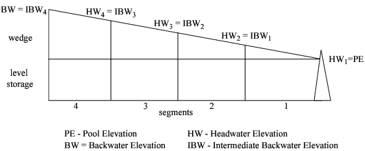
The Backwater Lambda LP Parameters (BLLPP) table is the only slot requiring user input, other than the physical data required to solve SlopePowerReservoirs with the Simulation controller. At least one realistic Headwater Elevation must be specified in the BLLPP table. Also at least one Inflow and/or Outflow for each segment is required, depending on the Reservoir’s configuration. The maximum and minimum Hydrologic Inflows during the run are automatically considered as potential Lambda Coefficients in addition to any user input Hydrologic Inflows in the BLLPP table. A lambda point is computed by RiverWare for every possible combination of Parameter values in the table columns. If a combination of values does not correspond to a feasible operational state, it is omitted from consideration. In certain cases, however, Inflow, Outflow, or Hydrologic Inflow values may not be required; the irrelevant columns in the BLLPP table are then omitted from the lambda point calculation. If any values are input into irrelevant columns, a warning message is issued at run time. The cases for which values are not required are:
Inflow is unnecessary if the a Profile Coeff Table parameter is zero for all segments. In this case, Inflow does not influence the backwater curve.
Outflow is unnecessary if the b Profile Coeff Table parameter is zero for all segments. In this case, Outflow does not influence the backwater curve.
Hydrologic Inflows are unnecessary if either the a or the wc Profile Coeff Table parameters are zero for all segments. In this case, Hydrologic Inflows do not influence the backwater curve. The minimum and maximum values are not treated as Lambda Coefficients.
The computed Lambda Points are stored in the Backwater Lambda Coefficients (BLC) table. The first columns of the table correspond to the Coefficients from the BLLPP table plus additional columns for time lagged Inflows and Outflows. The number of Inflow and Outflow columns is determined by the number of impulse response coefficients in the Profile Coeff Table. The remaining columns in the BLC table are the calculated Optimization parameters: Storage, Backwater Elevation, and Intermediate Backwater Elevations for each reservoir segment. Every row in the BLC table represents a valid lambda point. There is a row for each possible combination of Lambda Coefficients, including the lagged flows. The number of lambda point rows grows very quickly when multiple time lag columns compound the combinations. Since an excessive number of lambda points is unnecessary and affects performance, the number of lambda points is limited to 1,000.
The lambdaMethod uses the following slots in addition to those required for backwater calculation with the Simulation Controller:
Slots with Required Input Data
• Backwater Lambda LP Parameters (backwaterLambdaLPParms)
– TableSlot
– LENGTH, FLOW, FLOW, FLOW for each segment...
– valid operating points
– At least one Headwater Elevation is required. Inflow, Outflow, and Hydrologic Inflows may be required dependent on Reservoir configuration.
Slots with Output Data
• Backwater Lambda Coefficients (backwaterLambdaCoeffs)
– TableSlot
– LENGTH, FLOW for each irc..., FLOW for each irc..., FLOW for each segment..., LENGTH, LENGTH for each segment-1..., VOLUME
– a list of every combination of the valid operating points
Infeasible Solution Output File
RiverWare now automatically creates an output file when an infeasible optimization model is run. The file, called OPT_cplex_prob.*.iis, contains the “irreducibly inconsistent set” which represents the smallest infeasible problem from the failed run. This is typically a small set of inconsistent equations from which the erroneous constraint(s) can be deduced. The generation of this file is accompanied by a message window, indicating the exact name and path of the output file.
Optimization Output Files Directory
RiverWare-generated optimization files which begin with OPT_ are no longer saved in the RiverWare executable directory. All of these files, including those selected in the Optimization Controller Parameters dialog, are now saved in a sub-directory tree designed to facilitate management of this important debugging information.
The directory into which the files are saved is determined as follows:
• The top-most directory below which files are saved is either:
– the directory specified by the RiverWare_OPT_DIR environment variable,
– or the /tmp directory of the machine on which RiverWare is running.
Within this directory, a sub-directory is created as:
• the prefix “opt-” followed by the login name of the user.
(User johndoe would automatically generate a directory called opt-johndoe.)
Within this directory, an optional sub-directory may be created as:
• the File Directory: specified in the Optimization Controller Parameters dialog, if any.
For example: user johndoe running optimization with the RiverWare_OPT_DIR environment variable set to /RiverWare/Optimization, and the File Directory: set to run1, would generate OPT_ files as:
/RiverWare/Optimization/opt-johndoe/run1/OPT_*
If the File Directory: were then deselected, and the RiverWare_OPT_DIR environment variable were unset, OPT_ files would be generated as:
/tmp/opt-johndoe/OPT_*
In all cases, the directory to which optimization files are written is displayed as a green highlighted message in the Diagnostics Output Window.
Optimization Parameters Files
The PrsymOptParams file which contained optimization parameters for versions of PRSYM, has been divided into two files. The optimization parameters which are used exclusively by RiverWare are now contained in a file called goals.par. The optimization parameters which are required by the CPLEX solver are now contained in a file called cplex.par. The cplex.par file is passed directly to the solver as a command line argument, allowing a solution to be duplicated outside of the RiverWare executable. This is useful to access solver debugging capabilities which are unavailable during a RiverWare run.
The CPLEXPARFILE environment variable must be set as the path to the cplex.par file in order for this file to be located by the CPLEX solver. The path may be specified as an absolute path or a relative path from the directory set as the RiverWare_HOME environment variable.
Curvature Checks of Linearized Functions
Multiple term (MTLE & MTGE) Piecewise linearized functions are now checked for consistent curvature during Optimization runs. Violation of concavity or convexity is indicated by a warning message of the type:
SLOT(S): BlueRidge.Spill Bounds Linearization Table
“The value in row 48 column 1 (1796.703916) is outside the range of the approximation points and should be greater than the piecewise approximation (y = 9486.820540) for convex functions.”
The check to ensure that convexity or concavity is preserved is performed given the user approximation points, piecewise slopes, intercept, number of user approximation points, and the linearization context class of each table. The appropriate curvature is dependent upon the context, where MTLE and MTGE cases should yield convex and concave functions, respectively.
Two dimensional table values are checked by substituting the independent value into the piecewise function where the corresponding dependent value is computed. Since three-dimensional tables are linearized with respect to only one z point, their values are checked by examining independent values which are greater and less than the specified z point wherever an interpolation for the z approximation point is required. This provides a means with which to check for erroneous data which could potentially be used during actual interpolation. The appropriate independent values are then checked by substitution into the piecewise function where the corresponding dependent value is computed.
For both two-dimensional and three-dimensional tables, the dependent value is then compared to the table value to determine if the expected curvature is violated. In addition, piecewise slopes are checked relative to one another; convex and concave functions should yield slopes which are increasing and decreasing relative to one another, respectively.
Revised: 01/11/2023